Graph analytics on AMD GPUs using Gunrock#

Graphs and graph analytics are related concepts that can help us understand complex data and relationships. In this context, a graph is a mathematical model that represents entities (called nodes or vertices) and their connections (called edges or links). And graph analytics is a form of data analysis that uses graph structures and algorithms to reveal insights from the data.
Graph analytics can be used for various purposes, such as social network analysis, fraud detection, supply chain optimization, and search engine optimization. Graph analytics can also help us measure the importance, influence, similarity, and structure of the entities and their relationships.
Can AMD GPUs help with graph analytic operations? We will show some cases where GPUs can improve the performance of these valuable algorithms.
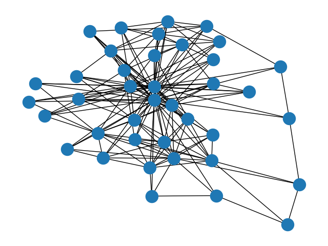
Figure 1: Visualization of the "chesapeake" dataset, a graph with 34 nodes and 340 edges.
The world of graph algorithms#
Now that we know that graphs are awesome, how do we analyze these complex data and relationships and find useful information from them? That’s where graph algorithms come in handy. Graph algorithms are 46 recipes that tell us how to cook up some insights from graphs. There are many types of graph algorithms that can do different things, such as:
Shortest Path algorithms: These algorithms help us find the quickest or cheapest way to get from one node to another in a graph.
Minimum Spanning Tree algorithms: These algorithms help us find a set of edges that connects all nodes in a graph with the lowest total weight.
Maximum Flow algorithms: These algorithms help us find the maximum amount of flow that can be sent from a source node to a sink node in a network.
Network Flow algorithms: These algorithms help us find the best way to match or assign nodes or resources in a bipartite graph.
Connectivity algorithms: These algorithms help us find whether two nodes are connected or reachable in a graph, or how many connected components are there in a graph.
Coloring algorithms: These algorithms help us assign colors to nodes or edges in a graph such that no two adjacent nodes or edges have the same color.
In this article, we will look in detail at a search algorithm known as Breadth-First Search (BFS) as a case study to help us learn more about graphs and graph analytics on GPUs.
Breadth-First Search, an introduction#
Breadth-First Search (BFS) is an algorithm for searching a tree or graph data structure for a node that satisfies a given property.
It starts at the root node and explores all the neighboring nodes
Then, it selects the nearest node and explores all the unexplored nodes
It often uses a queue data structure to keep track of the nodes to be visited
It also marks each node as explored or unexplored to avoid visiting the same node twice
BFS can find the shortest path from the root node to any other node in the graph

Figure 2: Visualization of BFS iterations operating on different levels of a graph.
How do I implement BFS?#
Let’s first start with a pseudocode. The BFS pseudocode below visits all the vertices of a graph in breadth-first order by placing the vertex into a queue, \(Q\), marking it as visited, and visiting all its neighbors. Each visited vertex is marked as “visited” to avoid processing the same vertex again. This process is repeated until all vertices have been visited (and the queue is empty). Simple!
BFS(graph, root):
    create a queue Q
    enqueue root onto Q
    mark root as visited
    while Q is not empty:
        current_vertex = dequeue Q
        for each neighbor of current_vertex:
            if neighbor is not visited:
                mark neighbor as visited
                enqueue neighbor onto Q
What can I do with BFS, a graph and a dream?#
BFS is a versatile algorithm with many applications in different domains. Some of them are:
Finding the shortest path and minimum spanning tree for unweighted graphs,
Finding all nodes within a given distance from a source node in a social network,
Finding the best move in a game tree by exploring all possible moves,
Crawling web pages by following links from a source page,
As a subroutine of more complex graph algorithms!
Within the Python ecosystem, frameworks like NetworkX provide convenient interfaces for building a variety of graph applications. For the BFS algorithmm, you can view the NetworkX Python implementation here. Now that we have defined the scope for the BFS algorithm, let us consider implementation on the GPU.
We can do better: AMD GPUs and Gunrock#
A wide variety of applications in HPC and AI have had remarkable successes using GPU acceleration. However, applying GPUs to problems in graph analytics remains a significant challenge. While GPUs are excellent in their ability to handle data parallelism spread out across a single-instruction set (single instruction multiple data a.k.a SIMD parallelism), graph applications often have multiple branching conditions and irregular memory access patterns, which pose a serious challenge. As a result, graph applications on GPUs often suffer from suboptimal GPU utilization and workload imbalances across wavefronts/warps. If that was not enough, certain graph algorithms require costly synchronization and communication between threads, which is amplified as the graph size increases.
The irregular and unpredictable nature of memory access patterns in graph algorithms can frequently lead to cache misses. With limited fast-chip memory, such as shared memory and thread-private registers, it is impractical to fit all the data necessary for processing large graphs and requires repeated requests to slower global memory. This will incur latency penalties that will greatly outweigh the high memory bandwidth GPUs provide and drastically reduce kernel performance. To get around these challanges, graph application code often requires intricate and complex modifications to compute kernels in order to handle these difficulties.
GPU accelerated graph analytics made easy and programmable#
Now that have a good sense of what GPU architecture looks like, we can leverage the massive parallelism available within the GPUs for graph analytics. Graph vertices and edges (millions or more of them) are a great fit for the massive parallelism and memory bandwidth available within modern GPUs. Researchers have proposed various programming abstractions which make the process of implementing graph algorithms and holistically thinking about parallel graph algorithms easier. Some of which include bulk-synchronous, asynchronous, data-centric, sparse-linear algebra based and more.
Since this article focuses on BFS, we highlight that parallel Breadth-first search (BFS) on GPUs is a well studied topic and has evolved significantly over the years. To summarize, some of the notable works:
Harish and Narayanan proposed a quadratic GPU BFS mapped each vertex’s neighbor list to a thread
Hong et al. improved this by using virtual warps
Merrill et al.’s linear parallelization with adaptive load balancing had a substantial impact
Beamer et al. introduced a hybrid BFS for shared memory machines, while
Enterprise optimized direction, load balancing, and status checks
BFS-4K refined the virtual warp method to a per-iteration dynamic one, using dynamic parallelism for improved load balancing.
Importantly, most of these works attempt to figure out a possible way to parallelize and load-balance the available computation within the BFS traversal onto the GPUs. For example, one possible implementation could map all the active vertices to individual threads, another could map all active edges (or source, edge, neighbor tuple) to individual threads, etc
Gunrock’s abstraction for graph analytics#
To simplify the complexity of programming parallel graph algorithms, such as BFS, we can rely on frameworks such as Gunrock to leverage the power of GPUs to solve complex graph algorithms. Gunrock is a C+±based GPU graph library which imploys bulk-synchronous, data-centric programming model and abstraction. Simply, it means that instead of translating graphs into sparse-matrices and implementing graph algorithms using sparse-linear algebra, Gunrock considers them as a collection of vertices connected with edges (the data-centric view). The “active” vertices (or edges), where active implies that in that specific iteration they are ready to be processed, are arranged into buckets called frontiers. All the active vertices or edges within a frontier are processed in parallel using GPU threads (bulk-synchronous view). After every parallel step, the system/GPU synchronizes and this process iteratively continues until an algorithm has converged. There are few key things we can summarize from Gunrock’s programming model:
Graph algorithms are generally expressed as iterative convergent processes
Frontiers are active set of vertcies or edges being processed in a specific iteration
Parallel operators which run on GPUs, process these frontiers
We can chain together parallel operators to create complex graph algorithms
Available parallel operators and their descriptions can be found in Gunrock’s documentation: https://gunrock.github.io/gunrock/gunrock.wiki/Gunrock-Operators.html. We instead will focus on only one key operation which is required to implement BFS. It is called advance. The advance operator simply generates a new frontier (new active set of vertices or edges) from a current frontier by visiting the neighbors of the current frontier. The illustration below shows advance, where the current frontier contained vertices 1 and 4, and the output frontier (after advance) contained all the neighbors of vertices 1 and 4.
Our first parallel Breadth-First Search!#
To implement our first parallel Breadth-First Search, we refer back to the sequential implementation above and recognize that BFS is being performed in an iterative manner. The first iteration is effectively a frontier that contains the starting vertex (source vertex) of the algorithm, and advancing to all of the neighbors of the active vertex. In the next iteration, the neighbors now become the active frontier and we visit all their neighbors until we have traversed the entire graph. We modify our pseudocode to show this parallel BFS approach:
PARALLEL_BFS(graph, root):
    create input frontier I
    create output frontier O
    add root onto I
    mark root as visited
    while I is not empty:
        [parallel] for all vertices in I:
            for each neighbor of source:
                if neighbor is not visited:
                    mark neighbor as visited
                    add neighbor onto O
        swap(O, I)
The key difference between parallel and sequential approach is the [parallel] for that
now visits all vertices I in the input frontier, and loops through the neighbors for
each vertex in I, producing the output frontier O.
The hard part of the puzzle: load-balancing#
Graph algorithms often inherently have workload imbalance, where neighboring parallel threads processing different source vertices (parallel for in the pseudocode above) can have different amounts of work to process. For example, if we are processing a social network graph; the vertices in the graph are “users” and an edge exists between two “users” if they are “followers” in that social network. If two “users” with drastically different numbers of “followers” were assigned to neighboring threads, and these threads needed to be synchronized at the end of our bulk-synchronous programming model defined above; then the thread with very few number of “followers” to process will be waiting on the thread with lots of “followers” to process. This problem is known as the load imbalance problem and is one of the most difficult thing to address when performing graph analytics in parallel (specifically on the GPUs, which follow the SIMD/SIMT model).
Luckily for us, Gunrock hides the complexity of load-balancing and other challenging implementation
level details within parallel graph analytics, and exposes operator level interface (such as
advance operator) to express the graph algorithms. And we can run it on AMD GPUs to see the
performance difference versus one of the most common python-based networkx library graph library.
Understanding the programming stack#
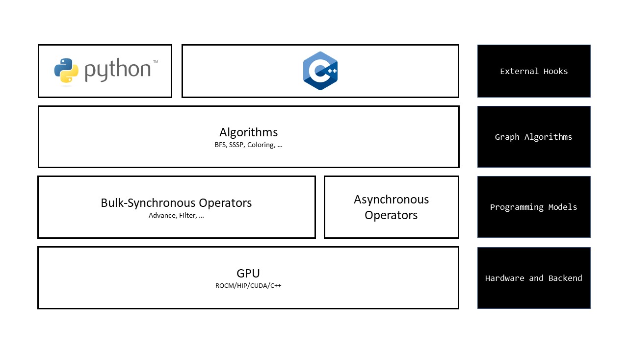
As implied in the previous section, Gunrock’s programming stack follows a “separation of concerns” philsophy, which separates its core programming models (such as the bulk-synchronous programming model described previously) from the low-level implementation details required to make graph alogorithms efficient on the GPU. In other words, Gunrock is written in a higher-level abstraction than hardwired implementations, leveraging reuse of its fundamental operators across different graph primitives. Applications using Gunrock can interface directly at the C++ level, or through a Python interface (not discussed here). An overview of supported graph primitives within Gunrock can be found here.
From python to C++/HIP#
The code below implements high-performant BFS (minus the boilerplate code), the two key
functions are the set-up phase: prepare_frontier and the loop phase: loop.
// Set-up the starting frontier.
void prepare_frontier(frontier_t* f,
                    gcuda::multi_context_t& context) override {
auto P = this->get_problem();
f->push_back(P->param.single_source);
}

// Execute this loop (on CPU) in a bulk-synchronous fashion
// till we have traversed the entire graph (output frontier is empty.)
void loop(gcuda::multi_context_t& context) override {

// User-provided root node to begin BFS.
auto single_source = P->param.single_source;

// Distances array to keep track of distances from root.
auto distances = P->result.distances;

// Visited array to mark vertices visited.
auto visited = P->visited.data().get();

// Define what should happen to each source, neighbor, edge and weight tuple
// on every step of the advance. This condition is applied in parallel.
auto search = [distances, single_source, iteration] __host__ __device__(
                    vertex_t const& source,    // ... source
                    vertex_t const& neighbor,  // neighbor
                    edge_t const& edge,        // edge
                    weight_t const& weight     // weight (tuple).
                    ) -> bool {
    // If the neighbor is not visited, update the distance. Returning false
    // here means that the neighbor is not added to the output frontier, and
    // instead an invalid vertex is added in its place. These invalides (-1 in
    // most cases) can be removed using a filter operator or uniquify.
    auto old_distance =
        math::atomic::min(&distances[neighbor], iteration + 1);
    return (iteration + 1 < old_distance);
};

// Launch advance operator on the above lambda function "search".
operators::advance::execute<operators::load_balance_t::block_mapped>(
    G, E, search, context);
}
Getting started with Gunrock for AMD GPUs#
Before building the HIP version of Gunrock, make sure your system has ROCm installed properly. Any version greater than 5 should be more than sufficient. We recommend readers consult the blog post on installing ROCm for a comprehensive overview. Installing the ROCm stack will also ensure library dependencies, such as rocPRIM and rocThrust, are available since these are required frameworks for the HIP build of Gunrock.
In addition to having ROCm installed, you will also need CMake version 3.20.1 or higher for configuration and building. Once these key dependencies are available on your system, you are ready to get started. The build instructions here assume you are using a Linux distribution, such as Ubuntu. Below is an example showing how to clone the Gunrock repository and compile for consumer graphics cards, such as the Radeon 6800XT or 6900XT. For our example, we specifically make an executable for running Gunrock’s BFS algorithms.
git clone -b hip-devel https://github.com/gunrock/gunrock.git
cd gunrock
mkdir build && cd build
cmake .. -DCMAKE_HIP_ARCHITECTURES=gfx1030  # change arch depending on the target device
make bfs  # or for all algorithms, use: make -j$(nproc)
Gunrock comes with a variety of
graph datasets ready for
experimenting with out of the box. To build all the datasets,
simply execute make in the datasets subdirectory of the
Gunrock project:
cd ../datasets
make
Once the datasets have been extracted, you can run
the bfs executable in the build/bin subdirectory and
provide the resulting .mtx data files:
cd ../build
bin/bfs ../datasets/chesapeake/chesapeake.mtx
For a complete list of argument options to the bfs executable, simply run bin/bfs --help.
Accelerating BFS: NetworkX versus Gunrock#
NetworkX is a Python package for graph analytics, which is easy to install, use, and experiment with. It is one of the most popular graph frameworks used by data scientists in Python, and it makes excellent use of the vibrant Python ecosystem for numerical linear algebra and data visualization. However, using GPUs through frameworks such as Gunrock even for basic graph traversal algorthms such as BFS can often result in significant boosts to performance for larger graph datasets.
To illustrate the impact of using AMD GPUs for accelerating graph workloads, we perform a simple comparison using the BFS algorithm from NetworkX (Python implementation) and Gunrock (HIP implementation) on a variety of datasets. The complete list of datasets featured in this comparison can be found in the Gunrock repository. The results collected using Gunrock were obtained using ROCm 5.7.1 and running on the Radeon 6900XT gaming GPU. The NetworkX calculations were obtained on an AMD EPYC 7742 64-Core Processor, though no parallelism was exploited in these experiments.
For all datasets, a random starting node was selected for each invocation of BFS (same across NetworkX and Gunrock results) and timing was averaged over a total of 25 iterations. The results for select datasets are presented in the table below.
Dataset |
Nodes |
Edges |
NetworkX (ms) |
Gunrock (ms) |
|---|---|---|---|---|
chesapeake |
39 |
340 |
0.097646 |
0.544522 |
webbase-1M |
1,000,005 |
3,105,536 |
10,975.20 |
2.94 |
hollywood-2009 |
1,139,905 |
113,891,327 |
64,862.21 |
9.93 |
roadNet-CA |
1,971,281 |
5,533,214 |
21,996.39 |
41.28 |
delaunay_n21 |
2,097,152 |
12,582,816 |
27,857.40 |
41.19 |
kron_g500-logn21 |
2,097,152 |
182,082,942 |
166,905.78 |
22.45 |
indochina-2004 |
7,414,866 |
194,109,311 |
146,979.89 |
1.17 |
delaunay_n24 |
16,777,216 |
100,663,202 |
251,753.90 |
116.38 |
road_usa |
23,947,347 |
57,708,624 |
309,478.87 |
328.47 |
Table 1: Comparison of average time (ms) for BFS to complete on different graph datasets using NetworkX and Gunrock. Dataset names, as well as the number of nodes/edges are provided.
The speed-ups observed are typical for this type of comparison and should not be generalized to frameworks using a parallel CPU implementation of BFS. For small datasets, such as the chesapeake graph, there is no real advantage to using GPUs. However, for datasets with several millions of nodes and edges, the difference in performance is very significant, resulting in a speed-up of several orders of magnitude just by switching to Gunrock’s GPU implementation.
Conclusion#
Graph analytics is an important tool for analysis of complex data, and graphs are ubiquituous across a wide variety of applications. If you are a data scientist working with interesting graph problems and datasets, in this blog we show that using Gunrock to take advantage of the AMD GPU in your system and get considerable performance benefits when processing large graphs through parallel graph analytics. If you have any questions or comments, please reach out to us on GitHub Discussions.
Acknowledgements#
The authors would like to acknowledge the great work done by Atharva Gondhalekar, a Ph.D. student in the Department of Electrical and Computer Engineering at Virginia Tech under the supervision of Prof. Wu Feng. During his time as a co-op in the Data Center GPU Software Solutions group, Atharva ported the Gunrock graph operators to HIP, which enabled Gunrock to run on AMD GPUs.