Using LoRA for efficient fine-tuning: Fundamental principles#

5, Feb 2024 by .
Low-Rank Adaptation of Large Language Models (LoRA) is used to address the challenges of fine-tuning large language models (LLMs). Models like GPT and Llama, which boast billions of parameters, are typically cost-prohibitive to fine-tune for specific tasks or domains. LoRA preserves pre-trained model weights and incorporates trainable layers within each model block. This results in a significant reduction in the number of parameters that need to be fine-tuned and considerably reduces GPU memory requirements. The key benefit of LoRA is that it substantially decreases the number of trainable parameters–sometimes by a factor of up to 10,000–leading to a considerable decrease in GPU resource demands.
Why LoRA works#
Pre-trained LLMs have a low “intrinsic dimension” when they are adapted to a new task, which means that data can be effectively represented or approximated by a lower-dimensional space while retaining most of its essential information or structure. We can decompose the new weight matrix for the adapted task into lower-dimensional (smaller) matrices without losing a lot of important information. We achieve this by low-rank approximation.
The rank of a matrix is a value that gives you an idea of the matrix’s complexity. A low-rank approximation of a matrix aims to approximate the original matrix as closely as possible, but with a lower rank. A lower-rank matrix reduces computational complexity, and thus increases the efficiency of matrix multiplications. Low-rank decomposition refers to the process of effectively approximating matrix A by deriving low-rank approximations of A. Singular value decomposition (SVD) is a common method for low-rank decomposition.
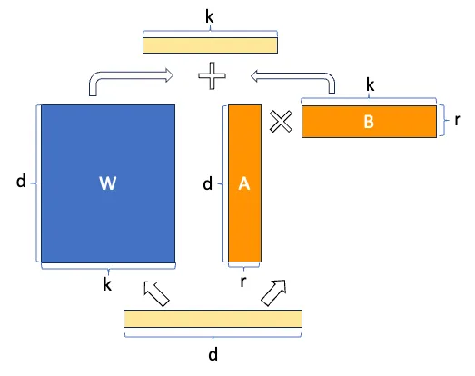
Suppose W represents the weight matrix in a given neural network layer and suppose ΔW is the
weight update for W after a full fine-tuning. We can then decompose the weight update matrix ΔW
into two smaller matrices: ΔW = WA*WB, where WA is an A × r-dimensional matrix, and WB is an
r × B-dimensional matrix. Here, we keep the original weight W frozen and only train the new
matrices WA and WB. This summarizes the LoRA method, which is also illustrated in the following
figure.
The benefits of LoRA#
Reduced resource consumption. Fine-tuning deep learning models typically requires substantial computational resources, which can be expensive and time-consuming. LoRA reduces the demand for resources while maintaining high performance.
Faster iterations. LoRA enables rapid iterations, making it easier to experiment with different fine-tuning tasks and adapt models quickly.
Improved transfer learning. LoRA enhances the effectiveness of transfer learning, as models with LoRA adapters can be fine-tuned with fewer data. This is particularly valuable in situations where labeled data are scarce.
Broad applicability. LoRA is versatile and can be applied across diverse domains, including natural language processing, computer vision, and speech recognition.
Lower carbon footprint. By reducing computational requirements, LoRA contributes to a greener and more sustainable approach to deep learning.
Train a neural network using the LoRA technique#
In this blog, we utilize the CIFAR-10 dataset to train a basic image classifier from scratch using several epochs. Following that, we further train the model with LoRA, illustrating the advantages of incorporating LoRA into the training process.
Setup#
This demo was creating using the following settings. For comprehensive support details, please refer to the ROCm documentation.
Hardware & OS:
Ubuntu 22.04.3 LTS
Software:
Getting started#
Import the packages.
import torch
import torchvision
import torchvision.transforms as transforms
Load the dataset and set the device.
# 10 classes from CIFAR10 dataset
classes = ('airplane', 'automobile', 'bird', 'cat', 'deer', 'dog', 'frog', 'horse', 'ship', 'truck')

# batch size
batch_size = 8

# image preprocessing
preprocessor = transforms.Compose(
    [transforms.ToTensor(),
    transforms.Normalize((0.5, 0.5, 0.5), (0.5, 0.5, 0.5))])

# training dataset
train_set = torchvision.datasets.CIFAR10(root='./dataset', train=True,
                                        download=True, transform=preprocessor)
train_loader = torch.utils.data.DataLoader(train_set, batch_size=batch_size,
                                        shuffle=True, num_workers=8)
# test dataset
test_set = torchvision.datasets.CIFAR10(root='./dataset', train=False,
                                    download=True, transform=preprocessor)
test_loader = torch.utils.data.DataLoader(test_set, batch_size=batch_size,
                                        shuffle=False, num_workers=8)

# Define the device
device = torch.device("cuda:0" if torch.cuda.is_available() else "cpu")
Display some samples from the dataset.
import matplotlib.pyplot as plt
import numpy as np

# helper function to display image
def image_display(images):
    # get the original image
    images = images * 0.5 + 0.5
    plt.imshow(np.transpose(images.numpy(), (1, 2, 0)))
    plt.axis('off')
    plt.show()

# get a batch of images
images, labels = next(iter(train_loader))
# display images
image_display(torchvision.utils.make_grid(images))
# show ground truth labels
print('Ground truth labels: ', ' '.join(f'{classes[labels[j]]}' for j in range(images.shape[0])))
Output:
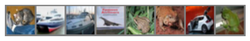
Ground truth labels: cat ship ship airplane frog frog automobile frog
Create a basic three-layer neural network for image classification, focusing on simplicity to clearly illustrate the LoRA effect.
import torch.nn as nn
import torch.nn.functional as F

class net(nn.Module):
    def __init__(self):
        super().__init__()
        self.fc1 = nn.Linear(3*32*32, 4096)
        self.fc2 = nn.Linear(4096, 2048)
        self.fc3 = nn.Linear(2048, 10)

    def forward(self, x):
        x = torch.flatten(x, 1)
        x = F.relu(self.fc1(x))
        x = F.relu(self.fc2(x))
        x = self.fc3(x)
        return x

# move the model to device
classifier = net().to(device)
Train the model.
We use cross-entropy loss and Adam for the loss function and optimizer.
import torch.optim as optim

def train(train_loader, classifier, start_epoch = 0, epochs=1, device="cuda:0"):
    classifier = classifier.to(device)
    classifier.train()
    criterion = nn.CrossEntropyLoss()
    optimizer = optim.Adam(classifier.parameters(), lr=0.001)

    for epoch in range(epochs):  # training loop

        loss_log = 0.0
        for i, data in enumerate(train_loader, 0):
            inputs, labels = data[0].to(device), data[1].to(device)
            # Resets the parameter gradients
            optimizer.zero_grad()

            outputs = classifier(inputs)
            loss = criterion(outputs, labels)
            loss.backward()
            optimizer.step()

            # print loss after every 1000 mini-batches
            loss_log += loss.item()
            if i % 2000 == 1999:
                print(f'[{start_epoch + epoch}, {i+1:5d}] loss: {loss_log / 2000:.3f}')
                loss_log = 0.0
Start to train the model.
import time

start_epoch = 0
epochs = 1
# warm up the gpu with one epoch
train(train_loader, classifier, start_epoch=start_epoch, epochs=epochs, device=device)

# run another epoch to record the time
start_epoch += epochs
epochs = 1
start = time.time()
train(train_loader, classifier, start_epoch=start_epoch, epochs=epochs, device=device)
torch.cuda.synchronize()
end = time.time()
train_time = (end - start)

print(f"One epoch takes {train_time:.3f} seconds")
Output:
    [0,  2000] loss: 1.987
    [0,  4000] loss: 1.906
    [0,  6000] loss: 1.843
    [1,  2000] loss: 1.807
    [1,  4000] loss: 1.802
    [1,  6000] loss: 1.782
    One epoch takes 31.896 seconds
It takes around 31 seconds for one epoch.
Save the model.
model_path = './classifier_cira10.pth'
torch.save(classifier.state_dict(), model_path)
We will train the same model with LoRA applied later and check how long it takes to train with one epoch.
Load the saved model and have a quick test.
# Prepare the test data.
images, labels = next(iter(test_loader))
# display the test images
image_display(torchvision.utils.make_grid(images))
# show ground truth labels
print('Ground truth labels: ', ' '.join(f'{classes[labels[j]]}' for j in range(images.shape[0])))

# Load the saved model and have a test
model = net()
model.load_state_dict(torch.load(model_path))
model = model.to(device)
images = images.to(device)
outputs = model(images)
_, predicted = torch.max(outputs, 1)

print('Predicted: ', ' '.join(f'{classes[predicted[j]]}'
                            for j in range(images.shape[0])))
Output:
Ground truth labels:  cat ship ship airplane frog frog automobile frog
Predicted:  deer truck airplane ship deer frog automobile bird
We observe that training the model for only two epochs does not produce a satisfactory outcome. Let’s examine how the model performs on the entire test dataset.
def test(model, test_loader, device):
    model=model.to(device)
    model.eval()
    correct = 0
    total = 0
    with torch.no_grad():
        for data in test_loader:
            images, labels = data[0].to(device), data[1].to(device)
            # images = images.to(device)
            # labels = labels.to(device)
            # inference
            outputs = model(images)
            # get the best prediction
            _, predicted = torch.max(outputs.data, 1)

            total += labels.size(0)
            correct += (predicted == labels).sum().item()

    print(f'Accuracy of the given model on the {total} test images is {100 * correct // total} %')

test(model, test_loader, device)
Output:
Accuracy of the given model on the 10000 test images is 32 %
This outcome suggests that there is significant potential to improve the model through further training. In the following sections, we will apply LoRA to the model and continue the training using this approach.
Apply LoRA to the model.
Define helper functions used to apply LoRA to the model.
class ParametrizationWithLoRA(nn.Module):
    def __init__(self, features_in, features_out, rank=1, alpha=1, device='cpu'):
        super().__init__()

        # Create A B and scale used in ∆W = BA x α/r
        self.lora_weights_A = nn.Parameter(torch.zeros((rank,features_out)).to(device))
        nn.init.normal_(self.lora_weights_A, mean=0, std=1)
        self.lora_weights_B = nn.Parameter(torch.zeros((features_in, rank)).to(device))
        self.scale = alpha / rank

        self.enabled = True

    def forward(self, original_weights):
        if self.enabled:
            return original_weights + torch.matmul(self.lora_weights_B, self.lora_weights_A).view(original_weights.shape) * self.scale
        else:
            return original_weights

def apply_parameterization_lora(layer, device, rank=1, alpha=1):
    """
    Apply loRA to a given layer
    """
    features_in, features_out = layer.weight.shape
    return ParametrizationWithLoRA(
        features_in, features_out, rank=rank, alpha=alpha, device=device
    )

def enable_lora(model, enabled=True):
    """
    enabled = True: incorporate the the lora parameters to the model
    enabled = False: the lora parameters have no impact on the model
    """
    for layer in [model.fc1, model.fc2, model.fc3]:
        layer.parametrizations["weight"][0].enabled = enabled
Apply LoRA to our model.
import torch.nn.utils.parametrize as parametrize
parametrize.register_parametrization(model.fc1, "weight", apply_parameterization_lora(model.fc1, device))
parametrize.register_parametrization(model.fc2, "weight", apply_parameterization_lora(model.fc2, device))
parametrize.register_parametrization(model.fc3, "weight", apply_parameterization_lora(model.fc3, device))
Now, our model’s parameters comprise two parts: the original parameters and the parameters introduced by LoRA. As we have not yet trained this updated model, the LoRA weights are initialized in a manner that should not impact the model’s accuracy (refer to ‘ParametrizationWithLoRA’). Therefore, disabling or enabling LoRA should result in the same accuracy for the model. Let’s test this hypothesis.
enable_lora(model, enabled=False)
test(model, test_loader, device)
Output:
Accuracy of the network on the 10000 test images: 32 %
enable_lora(model, enabled=True)
test(model, test_loader, device)
Output:
Accuracy of the network on the 10000 test images: 32 %
That’s what we expected.
Now let’s take a look how many parameters were added by LoRA.
total_lora_params = 0
total_original_params = 0
for index, layer in enumerate([model.fc1, model.fc2, model.fc3]):
    total_lora_params += layer.parametrizations["weight"][0].lora_weights_A.nelement() + layer.parametrizations["weight"][0].lora_weights_B.nelement()
    total_original_params += layer.weight.nelement() + layer.bias.nelement()

print(f'Number of parameters in the model with LoRA: {total_lora_params + total_original_params:,}')
print(f'Parameters added by LoRA: {total_lora_params:,}')
params_increment = (total_lora_params / total_original_params) * 100
print(f'Parameters increment: {params_increment:.3f}%')
Output:
    Number of parameters in the model with LoRA: 21,013,524
    Parameters added by LoRA: 15,370
    Parameters increment: 0.073%
The LoRA only adds 0.073% parameters to our model.
Continue to train the model with LoRA
Before we continue to train the model we want to freeze all the model’s original parameters as the paper mentioned. By doing this we only update the weights introduced by LoRA, which is 0.073% of the amount of the original model’s parameters.
for name, param in model.named_parameters():
    if 'lora' not in name:
        param.requires_grad = False
Continue to train the model with LoRA applied.
# make sure the loRA is enabled
enable_lora(model, enabled=True)

start_epoch += epochs
epochs = 1
# warm up the GPU with the new model (loRA enabled) one epoch for testing the training time
train(train_loader, model, start_epoch=start_epoch, epochs=epochs, device=device)

start = time.time()
# run another epoch to record the time
start_epoch += epochs
epochs = 1
import time
start = time.time()
train(train_loader, model, start_epoch=start_epoch, epochs=epochs, device=device)
torch.cuda.synchronize()
end = time.time()
train_time = (end - start)
print(f"One epoch takes {train_time} seconds")
Output:
    [2,  2000] loss: 1.643
    [2,  4000] loss: 1.606
    [2,  6000] loss: 1.601
    [3,  2000] loss: 1.568
    [3,  4000] loss: 1.560
    [3,  6000] loss: 1.585
    One epoch takes 16.622623205184937 seconds
You may notice that it now only takes around 16 seconds to complete training for one epoch, which is approximately 53% of the time required to train the original model (31 seconds).
The decrease in loss signifies that the model has learned from updating the parameters introduced by LoRA. Now, if we test the model with LoRA enabled, the accuracy should be higher than what we previously achieved with the original model (32%). If we disable LoRA, the model should yield the same accuracy as the original model. Let’s proceed with these tests.
enable_lora(model, enabled=True)
test(model, test_loader, device)
enable_lora(model, enabled=False)
test(model, test_loader, device)
Output:
    Accuracy of the given model on the 10000 test images is 42 %
    Accuracy of the given model on the 10000 test images is 32 %
Test the updated model again with the previous images.
# display the test images
image_display(torchvision.utils.make_grid(images.cpu()))
# show ground truth labels
print('Ground truth labels: ', ' '.join(f'{classes[labels[j]]}' for j in range(images.shape[0])))

# Load the saved model and have a test
enable_lora(model, enabled=True)
images = images.to(device)
outputs = model(images)
_, predicted = torch.max(outputs, 1)

print('Predicted: ', ' '.join(f'{classes[predicted[j]]}'
                            for j in range(images.shape[0])))
Output:
    Ground truth labels:  cat ship ship airplane frog frog automobile frog
    Predicted:  cat ship ship ship frog frog automobile frog
We can observe that the new model performed better compared to the results obtained in step 6, demonstrating that the parameters have indeed learned meaningful information.
Conclusion#
In this blog post, we explore the LoRA algorithm, delving into its principles and implementation on AMD GPU with ROCm. We have developed a basic network and LoRA modules from scratch to demonstrate how LoRA effectively reduces trainable parameters and training time. We invite you to delve deeper by reading about Fine-tuning the Llama model with LoRA and Fine-tuning Llama on a single AMD GPU with QLoRA.
Disclaimers#
Third-party content is licensed to you directly by the third party that owns the content and is not licensed to you by AMD. ALL LINKED THIRD-PARTY CONTENT IS PROVIDED “AS IS” WITHOUT A WARRANTY OF ANY KIND. USE OF SUCH THIRD-PARTY CONTENT IS DONE AT YOUR SOLE DISCRETION AND UNDER NO CIRCUMSTANCES WILL AMD BE LIABLE TO YOU FOR ANY THIRD-PARTY CONTENT. YOU ASSUME ALL RISK AND ARE SOLELY RESPONSIBLE FOR ANY DAMAGES THAT MAY ARISE FROM YOUR USE OF THIRD-PARTY CONTENT.