CuPy and hipDF on AMD: The Basics and Beyond

CuPy and hipDF on AMD: The Basics and Beyond#

May 06, 2025 by Fabricio Flores.

3 min read. | 684 total words.

Applications & models

PyTorch, AI/ML

This blog introduces you to CuPy and hipDF, two GPU-oriented high-performance computing Python libraries. This blog will show you how to deploy CuPy and hipDF on AMD GPUs using ROCm, and demonstrate the advantages of CuPy and hipDF over their traditional CPU-orientated counterparts, NumPy and Pandas.

To allow you to experience the GPU-optimized computational efficiency and accuracy of the CuPy and hipDF libraries firsthand, this blog will take you through a real-world application of CuPy and hipDF, showing you how to use the libraries in a detailed financial analytics example, optimizing an investment portfolio following the Markowitz model.

For more details on hipDF and its installation, see the official documentation: ROCm Data Science and the hipDF installation instructions. Additional information can be found visiting the official hipDF Github Repository.

Note

Throughout this blog, you will see the term “cuDF” used for commands and package calls. This reflects the fact that hipDF adopts the well-known cuDF API on AMD hardware, ensuring compatibility and ease of use across various computing environments. This API compatibility enables existing cuDF workloads to be effortlessly transitioned to run on supported AMD devices, allowing you to use AMD’s ROCm platform for your data processing tasks.

Note

You can also make use of the command “import hipdf” instead of “import cudf”. hipDF modules can also be called with “hipdf.MODULE” instead of “cudf.MODULE”

You can find all the files you need to follow this blog and get started with CuPy and hipDF here: GitHub folder.

Requirements#

AMD GPU: See the ROCm documentation page for supported hardware and operating systems.
ROCm 6.4: See the ROCm installation for Linux for installation instructions.
Docker: See Install Docker Engine on Ubuntu for installation instructions.
hipDF: see hipDF installation. This blog uses Docker Compose along a custom Dockerfile for a consistent testing environment.

Running this blog#

Clone the repo and cd into the blog directory:

git clone https://github.com/ROCm/rocm-blogs.git
cd rocm-blogs/blogs/artificial-intelligence/cupy_hipdf_portfolio_opt

Build and start the container. For details on the build process, see the cupy_hipdf_portfolio_opt/docker/Dockerfile.
```
cd docker
docker compose build
docker compose up
```
Open http://localhost:8888/ in your browser and open the /src/cupy_hipdf_portfolio_opt.ipynb notebook.

You can follow along with this blog using the cupy_hipdf_portfolio_opt.ipynb notebook.

Introduction to CuPy: the basics#

In high-performance computing, CuPy emerges as a significant library, particularly for its array creation and manipulation capabilities, which are similar to those found in NumPy. CuPy facilitates the creation of multi-dimensional arrays, leveraging the power of GPUs to enhance computational speed and efficiency. A key aspect of CuPy’s design is its compatibility with NumPy, enabling fluid interchange of array objects between these two libraries. This interoperability is fundamental for scenarios where developers want to harness the GPU-accelerated performance of CuPy while maintaining the established structure and functionality of NumPy codebases.

You can start by exploring some of the basics in data manipulation and operations on CuPy:

Creating arrays#

CuPy arrays are very similar to NumPy arrays. To create a CuPy array, use:

import cupy as cp

x_gpu = cp.array([1,2,3])
print(x_gpu.device)
x_gpu

<CUDA Device 0>
array([1, 2, 3])

Array operations#

The main advantage of CuPy is its ability to perform calculations on the GPU:

# Adding two arrays on GPU
y_gpu = cp.array([4,5,6])
sum_xy_gpu = x_gpu + y_gpu
print(sum_xy_gpu.device)
sum_xy_gpu

<CUDA Device 0>
array([5, 7, 9])

# Dot product of two arrays on GPU
z_gpu = cp.dot(x_gpu, y_gpu)
print(z_gpu.device)
z_gpu

<CUDA Device 0>
array(32)

Transforming between CuPy and NumPy#

NumPy arrays can be easily converted to CuPy arrays and vice versa.

To retrieve the device associated with a particular array, use the device property of a CuPy array. This helps determine where a specific array resides when multiple GPUs are in use.

# CuPy to NumPy
array_cpu = cp.asnumpy(x_gpu)
print(type(array_cpu))
array_cpu

<class 'numpy.ndarray'>
array([1, 2, 3])

# NumPy to CuPy
array_gpu = cp.asarray(array_cpu)
print(type(array_gpu))
array_gpu

<class 'cupy.ndarray'>
array([1, 2, 3])

When to use CuPy?#

CuPy is particularly useful when dealing with large arrays where GPU acceleration can lead to significant improvements in performance. Many deep learning frameworks are compatible with CuPy, making it a good choice for GPU-accelerated data processing.

For more detailed information, operations, and functions, see the CuPy documentation.

Introduction to hipDF: the basics#

hipDF is a GPU DataFrame library for loading, joining, aggregating, filtering, and manipulating data. It offers a pandas-like API familiar to data engineers and data scientists, enabling them to accelerate their workflows without delving into HIP programming details.

It is designed to provide a familiar interface for those who are used to working with Pandas DataFrames, but with the added benefit of the accelerated computing power of GPUs. Central to hipDF is the ability to create and manipulate DataFrames by using GPUs to expedite data manipulation tasks, including sorting, filtering, and aggregating large volumes of data. This efficiency is beneficial in data-intensive fields such as big data analytics and data science. Furthermore, hipDF offers seamless compatibility with Pandas, allowing for an effortless transition between GPU-accelerated and CPU-based data processing.

Some of the hipDF basics for data manipulation and operations are:

Creating DataFrames#

Similar to Pandas, DataFrames are created in hipDF this way:

import cudf

df_gpu = cudf.DataFrame({
    'a':[1,2,3],
    'b':[4,5,6]
})
print(type(df_gpu))
df_gpu

<class 'cudf.core.dataframe.DataFrame'>

	a	b
0	1	4
1	2	5
2	3	6

Basic operations#

hipDF DataFrames support many of the operations that Pandas DataFrames do:

# Adding a new column
df_gpu['c'] = df_gpu['a'] +  df_gpu['b']
print(type(df_gpu))
df_gpu

<class 'cudf.core.dataframe.DataFrame'>

	a	b	c
0	1	4	5
1	2	5	7
2	3	6	9

# Filtering based on a condition
filtered_df_gpu = df_gpu[df_gpu['c']>6]
print(type(filtered_df_gpu))
filtered_df_gpu

<class 'cudf.core.dataframe.DataFrame'>

	a	b	c
1	2	5	7
2	3	6	9

Conversion between hipDF and Pandas#

Converting between hipDF and Pandas is straightforward:

import pandas as pd

# hipDF to Pandas
df_pandas = df_gpu.to_pandas()
type(df_pandas)

pandas.core.frame.DataFrame

# Pandas to hipDF
df_gpu = cudf.DataFrame.from_pandas(df_pandas)
type(df_gpu)

cudf.core.dataframe.DataFrame

When to use hipDF?#

For high performance computing, hipDF is ideal for scenarios where the datasets fit into the GPU memory. hipDF performs extremely well on data science and analytics operations that are data-intensive, such as data filtering, aggregation, and group-by.

Performance comparison: NumPy vs CuPy#

The following example evaluates the performance gains when using CuPy over NumPy. It evaluates the processing time of an instruction that generates a 2D array of random numbers and computes its covariance matrix. Computing a covariance matrix is a well-known computationally intensive task.

Because GPU executions run asynchronously (tasks that run independently without blocking the program flow) with respect to CPU executions, use cupyx.profiler.benchmark instead of timing utilities, such as perf_counter, from the Python standard libraries. The cupyx.profiler.benchmark function is designed to measure the execution time of a function when running on different devices, like CPUs and GPUs.

Now see how these two libraries stack up against each other:

from cupyx.profiler import benchmark

# NumPy: generating a random matrix of size 500x1000 and computing its covariance

def generate_covariance_matrix(size):

    A_np = np.random.normal(0,1,size = size)
    covariance_matrix_np = np.cov(A_np)

    return covariance_matrix_np

numpy_times = benchmark(generate_covariance_matrix, ((500,10000),),n_repeat=10).gpu_times
print(f'Processing time cpu: {np.mean(numpy_times)} seconds')

The CPU’s processing time is: Processing time cpu: 0.13314309997558593 seconds.

# CuPy: generating a random matrix of size 500x1000 and computing its covariance

def generate_covariance_matrix(size):

    A_gpu = cp.random.normal(0,1,size = size)
    covariance_matrix_gpu = cp.cov(A_gpu)

    return covariance_matrix_gpu

cupy_times = benchmark(generate_covariance_matrix, ((500,10000),),n_repeat=10).gpu_times
print(f'Processing time gpu: {np.mean(cupy_times)} seconds')

On the other hand, the GPU’s processing time is: Processing time gpu: 0.0019042999148368837 seconds.

This small example illustrates how much performance is gained when executing array operations on GPU. In this case, the output of benchmark includes the average time taken for the function to execute over all 10 runs.

For more information, see performance best practices on CuPy.

Performance comparison: Pandas vs hipDF#

Similar as before, consider a simple test to evaluate the gains in performance when using hipDF over Pandas. Because hipDF does not have a direct equivalent to cupyx.profiler, you must resort to the Python timing library timeit to measure execution times over a given number of rounds.

The following example calculates the processing time of an instruction that creates a DataFrame and performs filtering and a grouping operation. Filtering and pivoting DataFrames are the most frequent operations in Pandas.

import pandas as pd
import cudf
import numpy as np
import timeit

col_a = list(np.random.rand(1_000_000))
col_b = list(np.random.rand(1_000_000))

def operations_pandas(col_a, col_b):
    df = pd.DataFrame({'A':col_a, 'B':col_b})
    filtered_df = df[df['A']>0.5]
    aggregated_df = filtered_df.groupby('B').agg({'A':'mean'})

pandas_time = timeit.timeit(lambda: operations_pandas(col_a, col_b), number = 10)

print(f'Processing time cpu: {pandas_time/10} seconds')

The output using Pandas is: Processing time cpu: 0.35824210699647663 seconds

def operations_hipdf(col_a, col_b):
    df = cudf.DataFrame({'A':col_a, 'B':col_b})
    filtered_df = df[df['A']>0.5]
    aggregated_df = filtered_df.groupby('B').agg({'A':'mean'})

hipdf_time = timeit.timeit(lambda: operations_hipdf(col_a, col_b), number = 10)

print(f'Processing time gpu: {hipdf_time/10} seconds')

While for hipDF the output is: Processing time gpu: 0.07872329596430064 seconds.

Like the case of measuring computation gain using CuPy, this test also considers the average execution time over 10 rounds using hipDF. You can observe the gains in performance when leveraging GPU processing power with operations using DataFrames.

Practical example: Markowitz model for optimal portfolio allocation#

You can now apply the tools that have been discussed through a hands-on exercise in applied finance, focusing on investment management and portfolio optimization. Specifically, this exercise explores the implementation of the Markowitz model. This model chooses a collection of financial assets that either maximizes return for a specific risk level or minimizes risk for a set return level. Central to the Markowitz model, also known as Modern Portfolio theory, is the concept of balancing a portfolio’s risk and return while taking into account the correlation between different assets.

To calculate the optimal portfolio allocation using the Markowitz model, you need to perform complex calculations, especially when dealing with extensive datasets. This is where leveraging high-performance computing tools like CuPy and hipDF becomes essential.

The Markowitz model is based on matrix operations that can be computationally intensive. CuPy is designed to efficiently handle these large matrix calculations. At the same time, hipDF is an excellent tool for managing and manipulating the data required by the model.

The first step in the process is to gather data on various stocks, focusing on their daily closing prices. The code sample organizes this information into a hipDF DataFrame, setting the stage for the subsequent calculations.

# Importing packages

import yfinance as yf
import pandas as pd
import cupy as cp
import cudf

def read_tickers(file):
    with open(file, 'r') as f:
        tickers = f.readlines()
        
    tickers = [ticker.strip() for ticker in tickers]

    return tickers

# Text file with the ticker (symbol) of the 10 stocks we are interested in
stocks = read_tickers('../data/tickers.txt')

def download_data(start_date, end_date):
    data = {}
    
    for stock in stocks:
        ticker = yf.Ticker(stock)
        closing_prices = ticker.history(start=start_date, end=end_date)['Close']
        data[stock] = list(closing_prices.values)

    # hipDF DataFrame from python dictionary    
    data_gpu = cudf.DataFrame(data)

    return data_gpu

# Historical time window of data to acquire. Define START and END dates
start_date = '2015-01-01'
end_date = '2021-01-01'

# Inspect the dataset
dataset = download_data(start_date, end_date)
dataset.head()

	AMD	AAPL	MSFT	GOOGL	AMZN	BLK	ADM	LMT	MO	UPS
0	2.67	24.466446	40.452740	26.477501	15.4260	283.385864	40.545143	151.744217	28.050333	83.356232
1	2.66	23.777185	40.080746	25.973000	15.1095	276.053558	39.142200	148.588562	27.889944	81.687302
2	2.63	23.779421	39.492466	25.332001	14.7645	271.763855	38.370579	147.889938	28.056067	81.151108
3	2.58	24.112865	39.994225	25.257500	14.9210	277.515259	38.947353	149.797440	28.571583	81.906288
4	2.61	25.039335	41.170799	25.345501	15.0230	280.756378	38.378368	153.172867	29.052742	83.378891

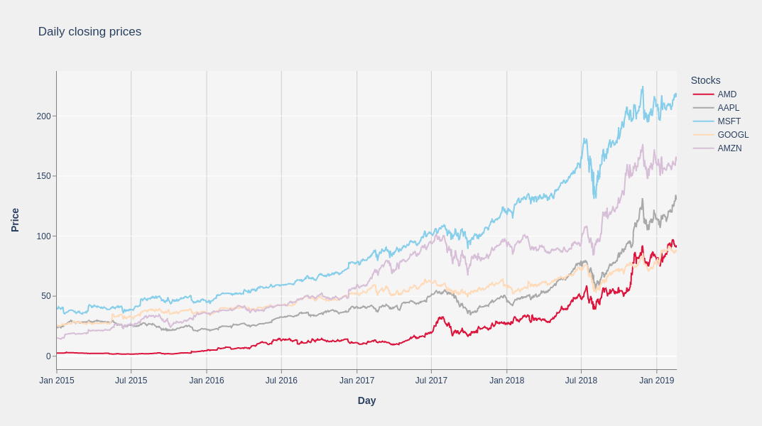
Portfolio of stocks: daily closing prices chart#

Now plot the closing prices of 5 of the 10 stocks you selected. For this purpose, you can use the Plotly library. Plotly is a Python graphing library for graphs and visualization. Because Plotly requires the data to reside on the CPU, you need to transform the hipDF series to NumPy arrays first.

import plotly.graph_objects as go
fig = go.Figure()

# Define some colors for each stock line
colors = ['crimson', 'darkgrey', 'skyblue', 'peachpuff', 'thistle']

for stock, color in zip(dataset.columns, colors):
    fig.add_trace(
        go.Scatter(
            x = cudf.date_range(start = start_date, end = end_date,freq = 'D').to_numpy(),
            y = dataset[stock].to_numpy(), 
            mode='lines', 
            name = stock, 
            line = dict(color = color)
        )
    )

fig.update_layout(
    title = 'Daily closing prices',
    xaxis_title = '<b>Day</b>',
    yaxis_title = '<b>Price</b>',
    legend_title = 'Stocks', 
    plot_bgcolor = '#f5f5f5',
    paper_bgcolor = '#f0f0f0',
)

fig.update_xaxes(showline = True, linecolor = 'gray', ticks = 'outside', tickcolor='gray', showgrid = True, gridcolor = '#d0d0d0')
fig.update_yaxes(showline = True, linecolor = 'gray', ticks = 'outside', tickcolor='gray', )

fig.show()

Closing prices

Compute the log returns of each asset#

This step computes the log returns. The reason for computing the log returns is to normalize the returns and treat gains and losses symmetrically. This step uses hipDF and CuPy together to take advantage of the CuPy array functionality. Start by performing a shift operation on the hipDF DataFrame followed by a point-wise division between DataFrames. The next step consists of removing empty (NULL) values from the hipDF DataFrame and then applying the natural logarithm operation to the resulting cuPy array:

# Interoperability between hipDF and cuPy arrays

# Compute returns on hipDF DataFrame
log_returns = dataset / dataset.shift(1)
log_returns = log_returns.dropna()

# hipDF DataFrame to cuPy and compute cuPy log of returns 
log_returns = cp.log((log_returns).to_cupy())
print(log_returns)

array([[-3.75234593e-03, -2.85760987e-02, -9.23831031e-03, ...,
        -2.10151623e-02, -5.73430788e-03, -2.02248087e-02],
       [-1.13422654e-02,  9.40106023e-05, -1.47861430e-02, ...,
        -4.71282032e-03,  5.93868707e-03, -6.58561807e-03],
       [-1.91945203e-02,  1.39249975e-02,  1.26251385e-02, ...,
         1.28156413e-02,  1.82077317e-02,  9.26282128e-03],
       ...,
       [-1.07562855e-02, -1.34041733e-02, -3.60729069e-03, ...,
        -7.90819348e-04, -1.82465555e-02, -1.36901989e-02],
       [ 1.82608336e-02, -8.56335307e-03, -1.10804072e-02, ...,
         7.34299514e-04,  2.45569605e-04, -1.67039550e-02],
       [-6.30438861e-03, -7.73240921e-03,  3.33263678e-03, ...,
         2.31273710e-03,  6.36184568e-03,  1.29698377e-02]])

Generate and plot the portfolios#

In the Markowitz model, generating random portfolios is essential to map out the efficient frontier, which represents the optimal balance of risk and return. This process lets you see the potential outcomes of various asset combinations, aiding in the selection of a portfolio that aligns with the risk tolerance and investment goals.

In this example, the function generate_portfolios_cp uses CuPy to generate a set of 10K random portfolios.

# Number of trading days in a year
NUM_TRADING_DAYS = 252

# The number of random portfolios to generate
NUM_PORTFOLIOS = 10000

def generate_portfolios_cp(returns):
    
    portfolio_means = []
    portfolio_risks = []
    portfolio_weights = []
    portfolio_sharpe_ratio = []

    for _ in range(NUM_PORTFOLIOS):

        w = cp.random.random(len(stocks))
        w /= cp.sum(w)
        
        # Append portfolio normalized weights
        portfolio_weights.append(w)
        
        # Calculate expected returns per asset
        mean_returns = returns.mean(axis = 0)
        
        # Portfolio total return
        portfolio_total_return = cp.sum(cp.asarray(mean_returns)*cp.asarray(w)) * NUM_TRADING_DAYS # 252 trading days in a year
        
        # Append portfolio total return
        portfolio_means.append(portfolio_total_return)
        
        # Calculate Covariance of returns
        covariance_returns = cp.cov(returns,rowvar = False)
        
        # cuPy for matrix multiplication
        # Append portfolio total risk(volatility)
        portfolio_total_risk = cp.sqrt(NUM_TRADING_DAYS*cp.dot(w.T, cp.dot(covariance_returns, w)))
        portfolio_risks.append(portfolio_total_risk)
        
        # Append sharpe ratio
        portfolio_sharpe_ratio.append(portfolio_total_return/portfolio_total_risk)
               
    return cp.array(portfolio_weights), cp.array(portfolio_means), cp.array(portfolio_risks), cp.array(portfolio_sharpe_ratio)

weights, means, risks, sharpe_ratios  = generate_portfolios_cp(log_returns)

Now you can plot the generated random portfolios:

def plot_portfolios(returns, volatilities, sharpe_ratios):
    fig = go.Figure(
        data = go.Scatter(
            x = volatilities,
            y = returns,
            mode='markers',
            marker = dict(color = sharpe_ratios, showscale = True, colorbar = dict(title = 'Sharpe Ratio'))
        )
    )
    
    fig.update_layout(
        title = 'Generated portfolios',
        xaxis_title = '<b>Expected Volatility</b>',
        yaxis_title = '<b>Expected Return</b>',
        plot_bgcolor = '#f5f5f5',
        paper_bgcolor = '#f0f0f0',
        height = 500
    )

    fig.update_xaxes(showline = True, 
                     linecolor = 'gray', 
                     ticks = 'outside', 
                     tickcolor='gray', 
                     showgrid = True, 
                     gridcolor = '#d0d0d0')
    
    fig.update_yaxes(showline = True, 
                     linecolor = 'gray', 
                     ticks = 'outside', 
                     tickcolor='gray')    
    
    fig.show()

plot_portfolios(cp.asnumpy(means), cp.asnumpy(risks), cp.asnumpy(sharpe_ratios))

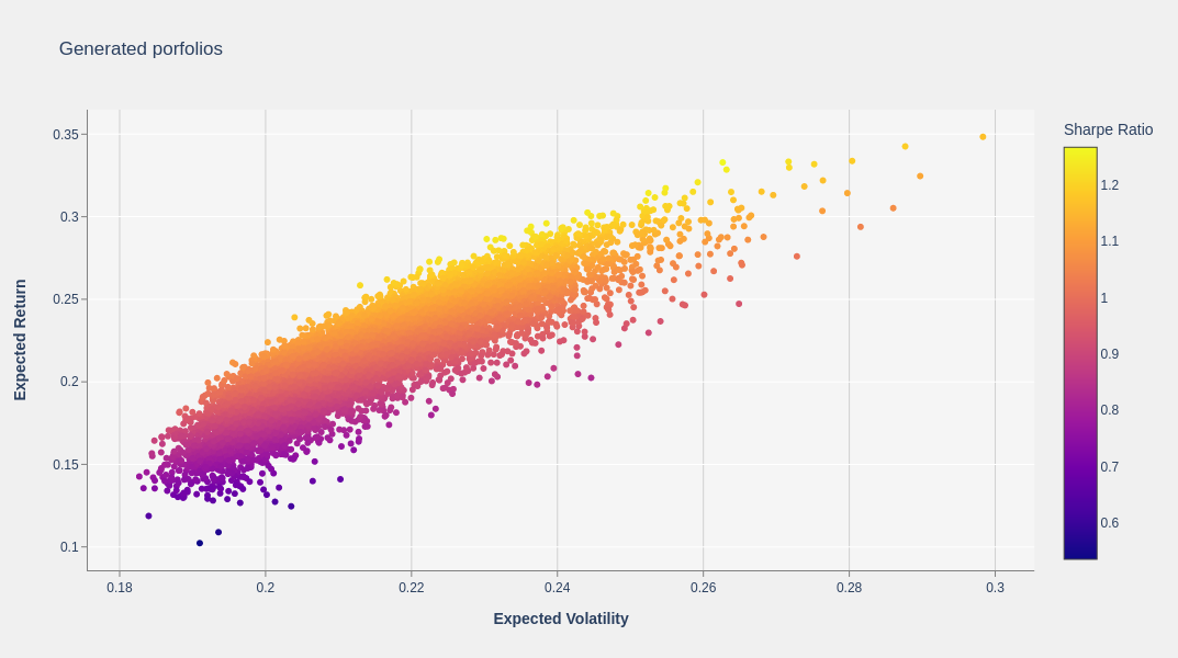
The next graph plots the resulting random portfolios from the Markowitz model. You can see a cloud of points, each representing a different portfolio with its own risk and return. Among these points, the most significant feature to look for is the Efficient Frontier.

The Efficient Frontier is the curved line along the upper boundary of this cloud of points. It represents the best possible return you can achieve for a given level of risk.

In summary, this plot demonstrates the trade-off between risk and return and guides investors to choose portfolios that maximize returns for a given risk appetite.

Generated portfolios

Get the optimal portfolio#

To find the optimal portfolio that offers the highest expected return for a given level of risk, use a metric called the Sharpe Ratio. The Sharpe Ratio helps determine how much excess return is received for the extra volatility of holding a riskier asset. A higher Sharpe Ratio indicates a more desirable investment.

In terms of identifying the optimal portfolio, the Sharpe Ratio is used to find the portfolio that offers the highest expected return for a given level of risk. Among the portfolios on the Efficient Frontier, the one with the highest Sharpe Ratio is considered the most efficient or optimal, because it yields the highest return per unit of risk.

With these considerations, select the portfolio that maximizes the Sharpe Ratio from the pool of generated portfolios. First, construct a hipDF DataFrame from the outputs of the generate_portfolios_cp function.

# Concatenate output values in a single array using CuPy

results = cp.concatenate([
    means.reshape(-1,1), 
    risks.reshape(-1,1),
    sharpe_ratios.reshape(-1,1),
    weights], axis = 1)

# Transform cuPy array to hipDF DataFrame
results_df = cudf.DataFrame(results, columns = ['Returns', 'Risk', 'Sharpe'] + [stock + "_weight" for stock in stocks])

The optimal portfolio in terms of the Sharpe Ratio is given by:

# Find portfolio with highest Shape Ratio
idxmax = results_df['Sharpe'].nlargest(1).index[0]
max_sharpe_portfolio = results_df.iloc[idxmax]
max_sharpe_portfolio

Returns         0.314794
Risk            0.246932
Sharpe          1.274819
AMD_weight      0.185692
AAPL_weight     0.155520
MSFT_weight     0.000681
GOOGL_weight    0.122865
AMZN_weight     0.263423
BLK_weight      0.038069
ADM_weight      0.008398
LMT_weight      0.202161
MO_weight       0.006247
UPS_weight      0.016946
Name: 5094, dtype: float64

You can also find the portfolio with the minimum risk and largest return as follows:

# Find the portfolio with the minimum risk(std dev)
idxmin = results_df['Risk'].nsmallest(1).index[0]
min_risk_portfolio = results_df.iloc[idxmin]
min_risk_portfolio

Returns         0.145790
Risk            0.182463
Sharpe          0.799009
AMD_weight      0.005347
AAPL_weight     0.014594
MSFT_weight     0.036912
GOOGL_weight    0.068934
AMZN_weight     0.156680
BLK_weight      0.056124
ADM_weight      0.147929
LMT_weight      0.188297
MO_weight       0.207179
UPS_weight      0.118004
Name: 3905, dtype: float64

Summary#

In this blog we introduced you to CuPy and hipDF and their deployment on AMD GPUs using ROCm. We showed you how to use CuPy and hipDF on AMD GPUs and demonstrated their significant advantages over their traditional, CPU-oriented counterpart libraries NumPy and Pandas in high-performance computing.

The blog also reflected on how CuPy excels in speed, particularly in large matrix operations, and how hipDF brings a seamless and significantly faster experience to Pandas workflows, without requiring code changes.

Finally, we demonstrated how combining CuPy and hipDF together can provide considerable advantages in high-performance computational tasks, through a practical, detailed example of deploying CuPy and hipDF in an investment portfolio allocation optimization using the Markowitz model running on AMD GPUs.

Disclaimers#

Third-party content is licensed to you directly by the third party that owns the content and is not licensed to you by AMD. ALL LINKED THIRD-PARTY CONTENT IS PROVIDED “AS IS” WITHOUT A WARRANTY OF ANY KIND. USE OF SUCH THIRD-PARTY CONTENT IS DONE AT YOUR SOLE DISCRETION AND UNDER NO CIRCUMSTANCES WILL AMD BE LIABLE TO YOU FOR ANY THIRD-PARTY CONTENT. YOU ASSUME ALL RISK AND ARE SOLELY RESPONSIBLE FOR ANY DAMAGES THAT MAY ARISE FROM YOUR USE OF THIRD-PARTY CONTENT.