Efficient Hyperparameter Optimization for Autonomous Driving Models with AMD Instinct GPU Partitioning#

For automotive OEMs and Tier-1 suppliers, developing production-grade perception models presents a significant bottleneck: achieving the accuracy required for safety-critical applications such as forward collision warning and autonomous emergency braking demands systematic hyperparameter optimization (HPO). However, HPO requires training hundreds of model variants, each taking hours on a single GPU, making thorough exploration of the parameter space prohibitively slow and expensive with conventional single-GPU setups.
We aim to address this challenge as part of an ongoing collaboration between AMD Silo AI and the Autoware Foundation, announced in December 2025 (for more details on the collaboration, see Advancing Open Autonomous Driving Perception at Scale). As part of this effort, we are accelerating Autoware’s end-to-end AI model training and deployment pipeline using AMD Instinct™ GPUs and ROCm™ software, uniting AMD’s scalable compute platform with Autoware’s open-source autonomous driving ecosystem - with a focus on optimizing Autoware’s perception models for production-grade Level 2+ autonomy targeting automotive OEMs, ensuring seamless performance from training to real-time inference.
By default, a single AMD Instinct™ MI300X exposes just 8 GPU devices, limiting parallelism. With GPU partitioning, the same AMD Instinct™ MI300X can be split into many more logical GPUs (up to 64), allowing a much higher number of parallel HPO workloads to run on a single node. In our experiments here, we show that GPU partitioning can accelerate HPO — all without requiring any changes to user code or additional programming effort — making high-quality, systematic optimization more economically viable for production AI pipelines.
AutoSpeed Overview#
AutoSpeed is a deep learning model for closest in-path object detection, designed for autonomous cruise control and advanced driver assistance systems. Its primary goal is to detect the closest object in the future driving path of the ego vehicle, supporting critical safety features such as forward collision warning and autonomous emergency braking.
The AutoSpeed network is a bounding box detection model inspired by the YOLOv11 architecture, but replaces the backbone c3k2 blocks with a custom-designed ‘context’ block for improved scene understanding. The model detects all foreground objects and classifies them into three categories based on their position relative to the predicted future driving path:
objects directly within the future driving path of the ego-car;
objects cutting-in/cutting-out of the future driving path;
objects outside of the future driving path.
The AutoSpeed model training described in the codebase uses a large set of hyperparameters, which have been set without any systematic tuning. By making efficient use of AMD GPUs to run many training jobs in parallel, we show here how hyperparameter optimization (HPO) can be applied to improve the quality of the model. Since HPO involves training many, slightly different models and training takes a substantial amount of time on a single GPU, we can improve the efficiency of the process by allowing a multi-GPU node to run many simultaneous jobs, sharing GPUs between multiple jobs. We do this using GPU partitioning.
Model Variants#
AutoSpeed is available in two main variants:
AutoSpeed 2.0: Processes frames in a 2:1 aspect ratio (512x1024 px), allowing detection of objects further away and providing a wider viewing angle. Recommended for new applications and developments.
Original AutoSpeed: Processes frames in a square aspect ratio (640x640 px).
This work has been done on the original AutoSpeed version (commit: 19d50518ff85dae56ffb2c66b59af7246ba15501).
The model is trained on the OpenLane dataset for the closest-in-path object (CIPO) detection task.
For more details, demo videos, and model weights, see the AutoSpeed repository.
OpenLane Dataset#
We have used the OpenLane dataset for experiments. OpenLane is the first large-scale, real-world 3D lane detection dataset, developed by OpenDriveLab. It contains 200,000 frames and over 880,000 carefully annotated lanes, collected from public perception datasets such as the Waymo Open Dataset. OpenLane provides both 2D and 3D lane annotations, as well as closest-in-path object (CIPO) and scene tags (weather, time, scenario), making it a comprehensive resource for autonomous driving research.
OpenLane provides a benchmark for 2D/3D lane detection. An evaluation kit is provided, including tools for evaluating both lane and CIPO detection following standard data formats and pipelines.
The dataset is distributed under the Creative Commons Attribution-NonCommercial-ShareAlike 4.0 license and is built on the Waymo Open Dataset, used under the Waymo Open Dataset License.
For the purposes of the experiments we present here, we use a subset of the OpenLane dataset: for training, the first of the 15 training segments, and for evaluation, the first of the three validation segments (see the numbered archives in the dataset distribution).
MI300X GPU Architecture and Partitioning#
The AMD Instinct™ MI300X GPU introduces a modular, scalable architecture optimized for high-performance computing (HPC), artificial intelligence (AI) and machine learning (ML) workloads. Key architectural features include:
8 XCDs (Accelerator Complex Dies): Each XCD contains 38 Compute Units (CUs), for a total of 304 CUs per GPU.
4 IODs (I/O Dies): Manage interconnects, memory, and data routing.
8 HBM (High Bandwidth Memory) stacks: 192GB unified HBM capacity, providing high memory bandwidth.
3D stacking: Each pair of XCDs is 3D-stacked on a single IOD for low-latency interconnects.
GPU partitioning allows the resources of a single GPU to be split between tasks, exposing the resources as if they were separate GPUs. The high memory capacity of the MI300X and the relatively low memory requirement of the AutoSpeed model mean that this is an effective way to make full use of the GPUs’ resources.
Dynamic compute partitioning is managed at the driver level and can be configured at runtime. The main partitioning modes are:
SPX (Single Partition X-celerator): The default mode (i.e. unpartitioned), exposes the entire GPU as a single device (304 CUs, 192GB HBM). Best for large models requiring unified resources.
DPX (Dual Partition X-celerator): Splits the GPU into two logical devices (each with 152 CUs, 96GB HBM). Useful for medium-sized models or balanced multi-tenancy.
QPX (Quadruple Partition X-celerator): Splits the GPU into four logical devices (each with 76 CUs, 48GB HBM). QPX is suitable for workloads that require more resources than CPX but less than DPX, offering a balance between resource allocation and concurrency for medium-sized models or multi-tenant scenarios.
CPX (Core Partitioned X-celerator): Splits the GPU into eight logical devices (each with 38 CUs, 24GB HBM). Ideal for multi-tenant environments, fine-grained scheduling and workloads that fit within a single XCD’s resources. Figure 1 shows how the GPU’s resources are split in CPX mode, compared to SPX.
Note: In practice, on some systems CPX mode may expose 63 logical devices, not 64.
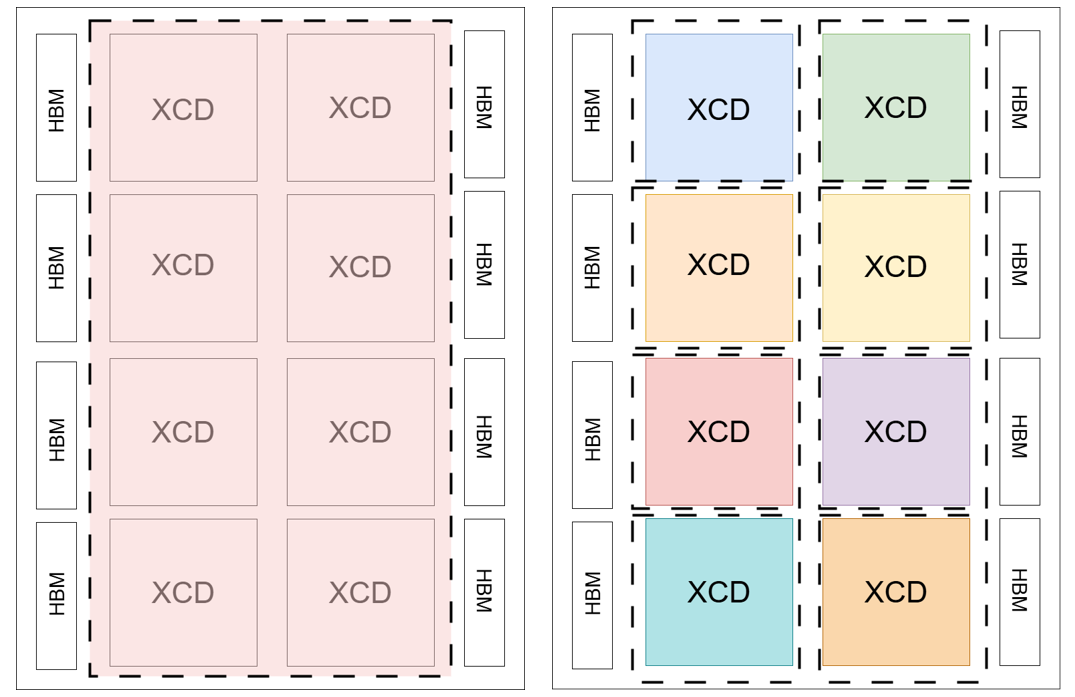
Figure 1: MI300X GPU partitioning modes. Left: SPX mode, all XCDs function as a single logical device. Right: CPX mode, each XCD operates as an independent logical device. Dotted lines indicate compute partition boundaries. Source: https://instinct.docs.amd.com/.#
To enable GPU compute partitioning, use the following command on your compute node. This requires root privileges and applies compute partitioning to all GPUs on the node:
sudo amd-smi set --gpu all --compute-partition <DPX/QPX/CPX/SPX>
Replace <DPX/QPX/CPX/SPX> with the desired partitioning mode. For more details, see the AMD Instinct™ MI300X GPU Partitioning Overview.
Model Performance Optimization#
To maximize the training efficiency and throughput of the AutoSpeed model, we applied several optimization strategies and compared the results in terms of the total compute throughput of an 8-GPU node.
PyTorch Profiler: Training performance was analyzed using the PyTorch profiler (enabled with
--do-profile), allowing for detailed inspection of CPU/GPU activity and bottlenecks. Profiling traces are saved for each run and can be visualized for further analysis.Data Preprocessing: Instead of decoding and resizing JPEG images on-the-fly during training, images are preprocessed into NumPy arrays ahead of time and stored on disk. These arrays are then loaded directly during training with the
--use-preprocessedflag, significantly reducing data loading overhead and improving training speed.Torch Compilation (
torch.compile): This feature, introduced in recent versions of PyTorch, uses ahead-of-time (AOT) compilation to optimize the model’s computation graph. By compiling model code into highly efficient kernels,torch.compilecan reduce Python overhead and fuse operations, resulting in faster training and inference. It is enabled in the training script with the--do-compileflag.Loss Vectorization: The loss computation was refactored to use vectorized operations instead of Python loops. This change leverages PyTorch’s optimized tensor operations, reducing the overhead of per-sample computations and improving overall training throughput. Vectorized loss functions are especially beneficial for large batch sizes and modern GPU architectures, as they maximize parallelism and hardware utilization.
These optimizations, especially data preprocessing, resulted in significant improvements in training speed and resource utilization, laying the groundwork for the throughput and HPO experiments described below.
Results#
Each optimization brings a substantial improvement in compute throughput. Here, compute throughput (FPS) is measured from per-batch training-step time after data is fetched, while overall/full workload throughput (FPS) is measured over end-to-end epoch time and therefore includes data loading and other host-side overhead. Vectorization and compilation both only bring a modest improvement when we look at the overall throughput, since the time taken by each iteration is dominated by slow data loading. Pre-processing brings a large improvement to both compute throughput and overall throughput. You can reproduce these results by running the optimization_comparison.sh script in the repository.
We get the highest throughput by combining all optimizations.
Run |
Compute throughput (FPS) |
Full throughput (FPS) |
|---|---|---|
Original |
241.23 |
117.36 |
Vectorized loss |
505.18 |
131.81 |
Pre-processing |
685.18 |
656.04 |
torch.compile |
485.09 |
132.12 |
All |
746.46 |
714.69 |
Requirements for Running the Experiments#
GPU Platform: AMD Instinct™ MI300X
ROCm™: Version 7.1 (recommended)
Docker®: Used for container builds
The repository includes a Dockerfile that allows you to quickly set up the necessary software environment for running experiments and the training pipeline. It also contains instructions on data preparation (using the unpack_data.sh script) and environment setup.
Throughput Experiment#
The throughput experiment measures the combined throughput from running multiple parallel training jobs — one per partition (e.g., SPX: 8 jobs, CPX: 63 jobs). We therefore run more jobs in total when using a higher degree of partitioning in order to test the scenario’s capacity for parallelisation. We report the total simultaneous throughput of the node under each setting.
These experiments can be reproduced using the run_partition_exp.sh script in the repository, which automates launching training jobs across all available logical GPUs for any given partitioning mode. In our experiments, disabling Automatic Mixed Precision (AMP) provided the best performance when using CPX and QPX partitioning.
Having configured GPU partitioning to one of the four available modes using sudo amd-smi set --gpu all --compute-partition <MODE>, we can start the Docker container and run run_partition_exp.sh. Complete results can be compiled from the logs of all training jobs using compare_throughput_experiments.py.
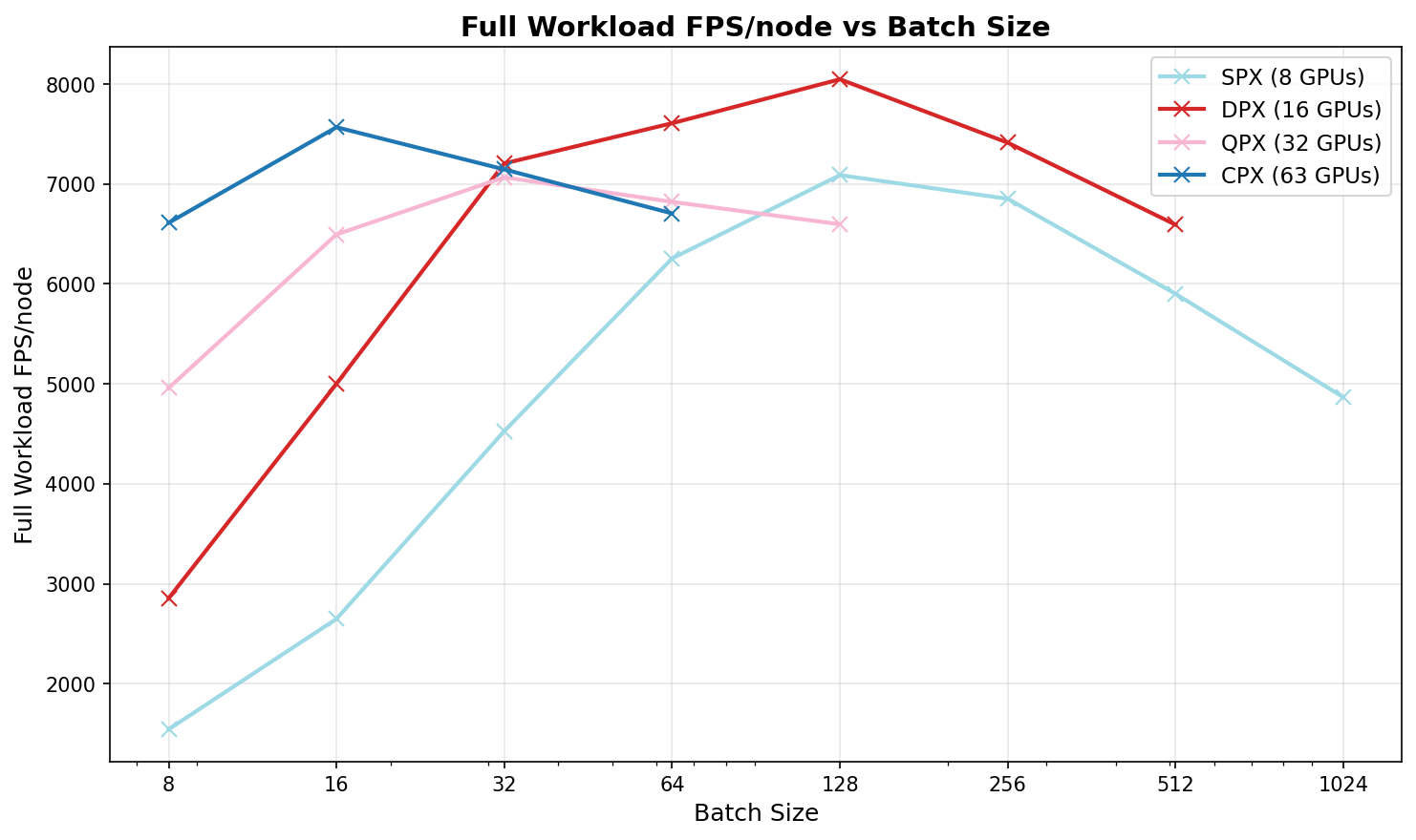
Figure 2: Comparison of the full workload FPS per node (8 GPUs) across partitioning modes. Missing points for higher batch sizes indicate out-of-memory failures.#
Figure 2 shows that all partitioning modes deliver a substantial throughput boost over the baseline (SPX, unpartitioned). For larger batch sizes, moderate partitioning (DPX, 16) offers the best results, while for smaller batch sizes, higher partitioning (CPX, 63) achieves the highest performance. Notably, SPX can accommodate larger batch sizes without running into out-of-memory (OOM) errors, whereas partitioned modes encounter OOM errors at lower batch sizes.
HPO Performance: Partitioned vs. Unpartitioned Nodes#
GPU partitioning significantly benefits HPO workloads by allowing multiple experiments to run in parallel, each on its own logical GPU and thus making fuller use of the available resources, especially where each model training job does not need the full resources of a whole GPU. The comparison above of throughput under different partitioning modes simulated the setting of an HPO study by simply running many AutoSpeed training jobs in parallel. Now we demonstrate the use of a sophisticated tool for HPO and show, with a small-scale HPO study, that CPX partitioning brings a substantial speedup in this more realistic setting.
For HPO experiments, we use batch size 32, the default for the AutoSpeed model. At batch size 32, the previous experiment showed similar results for all partitioning modes, CPX being preferred for lower batch sizes and DPX for higher. In the following HPO experiments, we compare CPX against SPX (unpartitioned) configurations.
For hyperparameter optimization (HPO), we used the Optuna framework, a Bayesian hyperparameter tuning library, to efficiently search the parameter space and manage experiment trials.
Running HPO with the Provided Optuna Script#
The repository includes an Optuna-based Python script (tune_autospeed_optuna.py) for orchestrating hyperparameter optimization (HPO) experiments on AutoSpeed, making use of all logical GPUs in the current partitioning mode.
Key Features#
Parallel trials: Each HPO trial is assigned to a separate logical GPU, enabling concurrent training and evaluation.
Flexible parameter ranges: Hyperparameter search spaces are defined in a YAML file, making it easy to customize the optimization process.
Progress tracking: The script provides real-time progress bars and logs to per-run files for monitoring trial and epoch completion.
Automatic resource management: GPU IDs are distributed to worker processes, ensuring each trial runs on a dedicated logical device.
Basic Usage#
Having prepared the training data in the same way as for the previous experiment, we can run HPO as follows, choosing a suitable number of trials and the number of training epochs we wish to use for each trial.
python tune_autospeed_optuna.py \
        --dataset /path/to/data \
        --hpo_ranges /path/to/hpo_ranges.yaml \
        --runs_dir /path/to/output_runs \
        --trials 20 \
        --epochs 5
Main Arguments#
--dataset: Path to the training dataset (e.g. OpenLane root directory).--hpo_ranges: Path to a YAML file specifying the hyperparameter search space (see below).--runs_dir: Directory where all trial outputs and logs will be saved.--trials: Number of HPO trials to run (default: 20).--epochs: Number of training epochs per trial (default: 5).--default_config(optional): YAML file with default config values for parameters not covered by the HPO search space.--optuna_db_location(optional): Directory for the Optuna database (default:/tmp/optuna).
How It Works#
The script creates a new Optuna study and output directory for each HPO run.
It detects the number of available GPUs (logical devices) and launches parallel worker processes, each bound to a specific GPU.
Each worker samples hyperparameters, trains the AutoSpeed model, evaluates performance, and logs results.
Progress is tracked live and the best configuration and metrics are reported at the end.
HPO Parameters#
The HPO ranges YAML file specifies ranges to be explored for each hyperparameter that is to be tuned. See the config file auto_speed.yaml in the AutoSpeed codebase for the full set of hyperparameters to the model and their default values.
min_lr:
    type: "loguniform"
    min: 1e-6
    max: 1e-4
box:
  type: "uniform"
  min: 5.0
  max: 10.0
cls:
  type: "uniform"
  min: 0.2
  max: 4.0
dfl:
  type: "uniform"
  min: 0.5
  max: 3.0
hsv_h:
  type: "uniform"
  min: 0.0
  max: 0.05
The HPO configuration supports three main categories of parameters:
Learning parameters: These include learning rate, optimizer settings, and related training hyperparameters.
Loss coefficient parameters: These control the weighting of different loss terms in the model (e.g.,
box,cls,dfl).Augmentation parameters: These define the strength and type of data augmentation applied during training (e.g., color jitter, geometric transforms).
You can specify ranges or fixed values for any parameter in your YAML file. The script will use any additional parameters defined in your YAML file as long as they are supported by the underlying training code.
Adjust the number of trials and epochs based on your available resources and desired search depth.
Optuna’s Sampling Algorithm and Parallelization Trade-offs#
By default, the Optuna framework uses TPESampler (Tree-structured Parzen Estimator), a Bayesian optimization algorithm that learns from previous trial results to inform the sampling of new hyperparameters. This means that when running multiple parallel trials, completed trials immediately contribute to the sampler’s probabilistic model, enabling pending jobs to benefit from accumulated knowledge.
Even though high parallelization could reduce the wall-clock time significantly, it limits the number of opportunities for the sampler to update its probabilistic model, since many trials are launched with the same prior information. This can make exploration less effective than with smaller, more frequent batches. For best results, ensure the total number of trials is much greater than the number of parallel workers. This ensures the sampler has sufficient sequential cycles to refine its search space, maximizing optimization quality.
Comparing HPO performance#
To compare unpartitioned (SPX) and partitioned (CPX) GPU parallelization, we run a study with 100 trials, training for just 5 epochs in each trial. For a real HPO study, we would want to set both of these parameters higher.
On a node with 8 MI300X GPUs, the complete HPO study finished in 3942.68s in SPX mode and 2678.23s in CPX mode, corresponding to a 1.47x speedup (47% faster) and about 32% lower runtime with GPU partitioning.
Note: Although CPX mode can expose up to 63 logical devices on an MI300X node, running HPO with this level of parallelism can become host-bound, potentially saturating CPU and memory. If this occurs, reduce parallel trial concurrency and dataloader workers, increase CPU/memory allocation, or use a less aggressive partition mode such as DPX.
HPO results#
In the above comparison, we ran only 5 epochs of each model training and only 100 trials (i.e. separate samples from the hyperparameter space). To find better hyperparameters, we need to run more trials, to make a more thorough exploration of the hyperparameter space, and train for longer, reflecting better how well each set of hyperparameters can be expected to perform.
Next, we run a more realistic (though still fairly modest) HPO study. We train each model for 15 epochs – only half the default full model training, but enough to have a good idea from the validation metrics of which model is most promising. We use the run_hpo.sh script.
We run HPO over seven hyperparameters: the optimizer parameters (min_lr, max_lr, momentum, weight_decay) and the loss component weights (box, cls, dfl). The exact ranges for each parameter can be found in the experiment1.yaml config file.
When tuning hyperparameters, it is essential to use a separate validation set to compute validation metrics for tuning, leaving assessment on the dataset’s main evaluation set until the final set of hyperparameters has been chosen. We therefore make a new 80/20 split of the training set to produce such a validation set.
Having run HPO, we can use the final, optimized hyperparameters to train a new AutoSpeed model on the full training set and test the model on the evaluation set. For comparison, we also train a model using the default hyperparameters. Both models are trained for 30 epochs.
P % |
R % |
MAP50 % |
MAP % |
|
|---|---|---|---|---|
Default params |
80.3 |
67.3 |
73.2 |
56.4 |
Optimized params |
84.1 |
69.0 |
75.4 |
57.7 |
HPO has led to a substantial improvement in all metrics.
It should be noted that these experiments have used only a portion of the training and test sets of OpenLane. To train a model for real use, one should use the full training set (split into training and validation sets for HPO, as here) and test set both for finding optimal hyperparameters and for training and testing the final model.
Summary#
AMD Instinct™ MI300X’s compute partitioning feature provides flexibility and efficiency for HPO and other multi-tenant workloads. By slicing the GPU into logical devices, users can achieve higher throughput and improved workload density — especially valuable for AutoSpeed and similar models requiring scalable parallelism and relatively modest resources for each job.
Future collaboration#
This blog represents an early milestone in the broader AMD Silo AI and Autoware Foundation collaboration. Looking ahead, the partnership plans to extend this work in several directions:
training and optimizing end-to-end driving models for point-to-point navigation in robotaxi applications;
integrating and optimizing photorealistic and physics-accurate Physical AI world models;
developing open MLOps pipelines for Physical AI applications in autonomous driving.
The joint commitment to open-source development means that results, tools, and best practices from this collaboration will continue to be shared with the community, supporting faster and safer autonomous driving innovation across OEMs, Tier-1 suppliers, and research institutions worldwide.
Acknowledgement#
This work has been supported by the EuroHPC JU project “MINERVA” (GA No. 101182737).
The experiments in this blog post used data from the OpenLane dataset, developed by OpenDriveLab and described in Chen et al., PersFormer: 3D Lane Detection via Perspective Transformer and the OpenLane Benchmark (ECCV 2022). OpenLane is licensed under the Creative Commons Attribution-NonCommercial-ShareAlike 4.0 International (CC BY-NC-SA 4.0) license. OpenLane is built on the Waymo Open Dataset and is also subject to the Waymo Dataset License Agreement for Non-Commercial Use. Anyone reproducing this work must comply with both licenses, including registering at the Waymo Open Dataset website and agreeing to the Waymo terms before downloading OpenLane. Access to, use of, and redistribution of the dataset or derivative works are governed by those licenses.
Additional Resources#
Disclaimers#
Third-party content is licensed to you directly by the third party that owns the content and is not licensed to you by AMD. ALL LINKED THIRD-PARTY CONTENT IS PROVIDED “AS IS” WITHOUT A WARRANTY OF ANY KIND. USE OF SUCH THIRD-PARTY CONTENT IS DONE AT YOUR SOLE DISCRETION AND UNDER NO CIRCUMSTANCES WILL AMD BE LIABLE TO YOU FOR ANY THIRD-PARTY CONTENT. YOU ASSUME ALL RISK AND ARE SOLELY RESPONSIBLE FOR ANY DAMAGES THAT MAY ARISE FROM YOUR USE OF THIRD-PARTY CONTENT.