A Step-by-Step Walkthrough of Decentralized LLM Training on AMD GPUs#

LLMs have shown great capability to generalize new tasks and are at the core of many AI applications recently. Performance of these models has scaled with model size, resulting in training of larger models on massive datasets. This increase in computation requirements has led to training of these LLMs on a huge number of GPUs and poses significant engineering and infrastructure challenges in ensuring standard backpropagation training. They are trained on a strongly interconnected network of devices and hence limit training of the models to a single cluster / data center.
In this blog, you will learn how decentralized training offers a practical alternative to this model. We walk through the fundamentals of decentralized LLM training, introduce the DiLoCo algorithm, and demonstrate how to run real training workloads using the Prime framework on AMD Instinct™ MI300 GPUs. By the end, you will understand how to scale LLM training beyond a single cluster, reduce communication overhead, and unlock underutilized GPU resources across geographically distributed environments.
Distributed and Decentralized Training Paradigms#
Most models are trained on a collection of GPUs in parallel, referred to as distributed training, with the most popular approaches being Distributed Data Parallel (DDP), Full Sharded Data Parallel (FSDP), etc. These are very effective and have helped push the boundaries and resulted in breakthroughs in training LLMs. However, the biggest limitation with this approach is that it requires the presence of a huge number of GPUs in a close radius such that the network bandwidth among the resources is maximized. This particularly requires huge investments in dedicated and localized datacenters as well as expensive and power-hungry networking infrastructure and prevents the use of resources which might already be present elsewhere.
This is where the concept of decentralized training comes in which aims to train models using several clusters, each hosting a small number of devices. These islands of devices are usually poorly connected and resemble scenarios where the data centers might be spread across continents. This allows one to increase the number of GPUs available as decentralized clusters enable aggregation of resources as well as enabling heterogenous devices across the clusters.
The most popular algorithm in this domain is the DiLoCo (Distributed Low Communication Training of Language Models), which is heavily inspired by the Federated averaging algorithm. Each cluster maintains a copy of the model and performs extensive independent training over many iterations (inner optimization), communicating with other clusters only after these inner steps during the outer optimization phase, thereby reducing the need for continuous inter-cluster communication. Formally the algorithm is as in Figure 1.
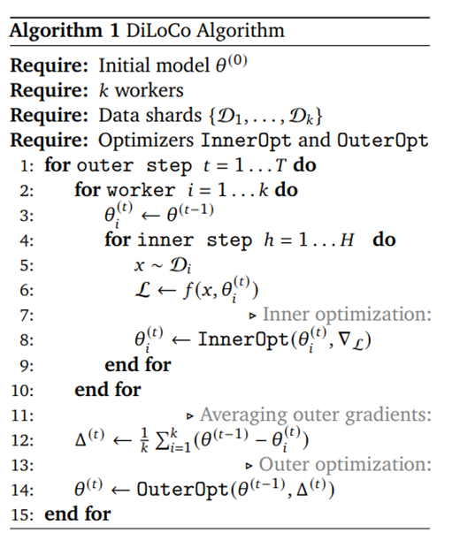
Figure 1: DiLoCo Algorithm.
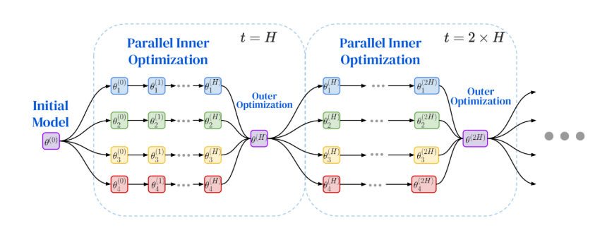
Figure 2: Visualisation of the DiLoCo algorithm.
The workers (4 in the example image provided) each start with the initial model with parameters (\(\theta\)), which could be either randomly initialized or a pretrained model. Every worker maintains its own shard of data, which means \(k\) workers would each have \(k\) shards of data.
The primary benefit of this training paradigm is that it requires communication only at the outer optimizations which take place only after a considerably large number of inner steps. Denoting the number of outer steps by \(T\) and the number of inner steps per outer step by \(H\), the total number of training iterations is \(T \cdot H\), while the number of communication events is \(T\) (rather than \(T \cdot H\), as in conventional synchronous distributed training). This reduction in communication frequency enables improved scalability to workers with limited or high-latency connectivity across geographically distributed locations.
OpenDiLiCo and Prime#
OpenDiLoCo is the open-source implementation of DiLoCo. They implemented the concept as well as reproduced the results from the paper. They employ some enhancements in the method particularly FSDP within the group, gradient compression from FP32 to FP16 and Hivemind for management of distributed systems. This was followed by the prime framework which is the production ready version of the previous. They retain the FSDP within the nodes from the previous while introducing new changes as shown below:
Parallel TCP stores among the GPUs with the same FSDP shard.
Gradient compression to INT8 from FP32.
Elastic Device Mesh for system management which implements heartbeat mechanism to detect failures.
In this blog we will discuss running the repository to train a Llama2 model using the Prime framework in a few different ways on the AMD Instinct™ MI300 GPUs. After which we will show our results for some sample runs further showcasing the usefulness of DiLoCo.
Getting started and setup for the repository#
The repository is located here AMD-AGI/prime_amd: Prime repository with functionality enabled on AMD
For an easy installation which will clone the repository and download some initial data, run the following command:
curl -sSL https://raw.githubusercontent.com/AMD-AGI/prime_amd/main/scripts/install/install.sh
Alternatively, you can follow the detailed instructions given below:
Clone the repository
git clone git@github.com:AMD-AGI/prime_amd.git
Download the dependencies
curl -LsSf https://astral.sh/uv/install.sh \| sh #download the uv
package manager

source $HOME/.local/bin/env #apply uv configs to the environment

sudo apt install iperf -y #download iperf server for determining pings
between clusters
Activate the env and download the packages
uv venv #create new uv virtual environment*

source .venv/bin/activate #activate the uv environment

uv sync --extra rocm --extra all #download the dependencies

git submodule update --init --recursive #download gloo
Login to wandb (optional- only if logging the results) and hugging face. A prompt would show up and enter your API keys for both the platforms.
wandb login #to upload training metrics

huggingface-cli login #to pull the tokeniser from hugging face
Download Data#
To conduct a quick experiment using synthetic data, you may skip this step and refer to the final entry in the sample configuration file.
Now that we have the environment setup and have activated the virtual environment, it is time to download some data. The data we use for this is the same as the original repository, fineweb-edu. We can download some shards of the data from hugging face to run our demo experiments.
python scripts/subset_data.py --dataset_name PrimeIntellect/fineweb-edu --data_rank 0
This will download around 300GB of the fineweb-edu dataset, you can reduce the data downloaded by setting the –max-shards to a custom value. The data can be downloaded to every node entirely, kept in a shared storage or just download the necessary data required for the particular node. The amount of data being downloaded can be controlled by further setting the –max_shards and –data_world_size.
Training Configurations#
The Llama2 model has already been defined in the train.py and we shall use that for our experiments currently. Now that we have the data, we can train a model from one of the various configuration files already present. In this case we will train a 150M model across 2 groups using the following configurations:
name_model = "150M" #training run name

project = "150m_prime_300"

type_model = "llama2" #type of base model to use, can switch between Llama2 and Llama3

[train]

micro_bs = 64 # change this base on the gpu

reshard_after_forward = false #if the model should be resharded after forward pass for FSDP

torch_profiler = false # if the runs have to be profiled

[optim]

batch_size = 256 #batch size of the particular group

warmup_steps = 1000 #optimizer warm up steps

total_steps = 88_000 #total pretraining steps

[optim.optim]

lr = 4e-4 #learning rate to use for the inner optimizer

[diloco]

inner_steps = 500 #DiLoCo merging should take place at the end of which step

compression= "uint8" #should the gradients be compressed during communication at DiLoCo step

[ckpt]

path = "/data/datasets/dilico/dilico_doubleGRP" #where to save the model checkpoints and at what intervals

interval = 44000

[data] #config if using real data

data_path="path to downloaded data"

[data] #config to include if using fake data, faster to get started

fake = true
Once we have the configuration file in place, we need to set the
environment variables, the variables are defined in setup_env.sh.
After completing the initial setup, it is now time to execute the command that initiates the training process.
Command on group 1:
GLOBAL_UNIQUE_ID=0 GLOBAL_RANK=0 PYTHONPATH=src torchrun --nproc_per_node=8 --node-rank 0 --rdzv-endpoint localhost:$((BASE_PORT + 0)) --nnodes=1 src/zeroband/train.py @configs/150M/MI300.toml --data.data_rank 0 --data.data_world_size 2
Command on group 2:
GLOBAL_UNIQUE_ID=1 GLOBAL_RANK=1 PYTHONPATH=src torchrun --nproc_per_node=8 --node-rank 0 --rdzv-endpoint localhost:$((BASE_PORT + 0)) --nnodes=1 src/zeroband/train.py @configs/150M/MI300.toml --data.data_rank 1 --data.data_world_size 2
If both the groups are on the same machine, the --rdzv-endpoint should
be set as localhost:$(BASE_PORT +1) on the second group to avoid
conflicts.
This will start training on both nodes.
The data.data_rank and data.data_world_size is a factor which depends on how you distribute the data across groups. In the example above, we have the exact same dataset downloaded across the 2 groups, in which case we define the world size as 2 and assign ranks to each group. This ensures that there isn’t any overlap of data between them. In the case that both the groups downloaded only data necessary to the group’s training, the data.data_world_size would be 1 and data.data_rank would be 0.
We trained the 150M model across different configurations on the AMD Instinct MI300 GPU and the results and observations are as follows:
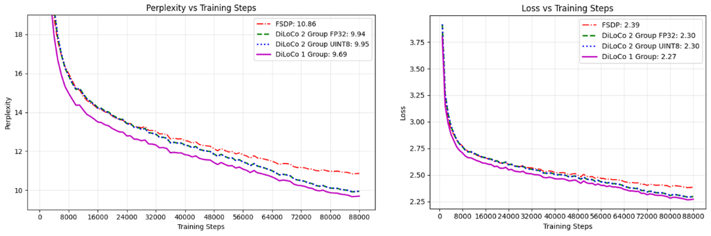
Figure 3: The DiLoCo setup attains lower perplexity and loss as opposed to equivalent FSDP training. Also, the gradient compression doesn’t have significant impact on the convergence.
The configurations we have piloted are the following, we have attempted to keep the comparisons fair by keeping the effective batch sizes to be the same along with keeping overall GPUs across all to be uniform:
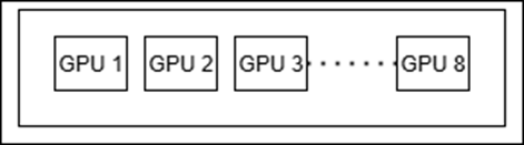
FSDP only:
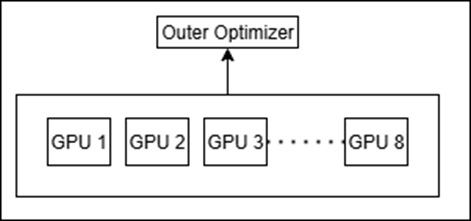
Figure 4: FSDP Setup.
DiLoCo with 1 group: This is similar to FSDP but the DiLoCo step at the end of the inner steps acts as a lookahead optimizer and updates the gradients of the model.
Figure 5: DiLoCo with 1 Group Setup.
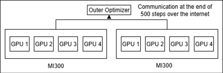
DiLoCo with 2 groups of 8 GPUs (one with compression of gradient and the other without): We mimic this setting on a single node through docker isolation, details of achieving this are given towards the end of the article.
Figure 6: DiLoCo with 2 Group Setup.
Our observations#
DiLoCo with 1 group as well as DiLoCo with 2 groups outperforms FSDP with the gap widening as the number of steps increases.
The compression performed during transmission of gradients from FP32 to Unsigned INT8 doesn’t have an impact on convergence or the results as the curves are nearly identical.
DiLoCo apart from being effective for decentralized training is also a viable new distributed training paradigm.
Some Tips#
Defining your own custom LLM#
In this tutorial we experimented with a predefined Llama model present
in the models folder. You can define your custom model instead and
get_model() in __init__.py should return your model along with the
config for the particular model. The model we are using is a
Transformer class derived from nn.Module and calls the transformer
layers in sequence. The implementation of the transformer can be altered
or completely changed to cater to a custom model.
The data the framework currently expects is in the form of multiple parquet files, any dataset to be used could be formatted in similar fashion.
Testing setup on a single Machine through Docker Isolation#
Sometimes, before we start training on a decentralized cluster, we may want to make sure our setup is working, for which purpose we can simulate the scenario on multiple docker images on the same machine. Each docker will only expose part of the GPUs to the image, and hence resembling a scenario of different machines over the internet.
To divide the GPUs on a machine, we first need to find its Direct rendering manager (DRM) number. It can be found for the GPUs on a machine using the following command:
$ cat /sys/class/kfd/kfd/topology/nodes/2/properties | grep drm_render_minor
drm_render_minor 128
You can search similarly for nodes 2 through 9 (assuming 8 GPUs per machine). They usually begin sequentially from 128, but this can vary. Once we have the DRMs for the GPUs, we can use a Docker run command as follows:
export WORKDIR=/home/user

export WORKSPACE_DIR=/home/user

export CONTAINER_NAME=mohbasit_4_gpus

export IMAGE_NAME=rocm/pytorch:latest

docker run \

--device=/dev/kfd \

--device=/dev/dri/renderD128 \

--device=/dev/dri/renderD129 \

--device=/dev/dri/renderD130 \

--device=/dev/dri/renderD131 \

-d \

--user root \

--network=host \

--ipc=host \

--workdir $WORKDIR -v $WORKSPACE_DIR:$WORKDIR --name
$CONTAINER_NAME $IMAGE_NAME \

tail -f /dev/null
Summary#
Decentralized training is rapidly emerging as a scalable alternative to traditional distributed learning. In this blog, you explored the DiLoCo algorithm step by step, understood how it reduces communication overhead through inner and outer optimization loops, and saw how this approach enables training across loosely connected or geographically distributed GPU clusters. Through hands-on walkthroughs, you gained practical experience setting up the Prime—the production ready implementation of DiLoCo—repository, preparing data, configuring training runs, and launching decentralized training jobs on AMD Instinct™ MI300 GPUs. You saw concrete experimental results comparing FSDP and DiLoCo configurations, showcasing how it not only reduces communication overhead but can match or even exceed the performance of standard FSDP-based training. Overall, this blog equipped you with both the conceptual foundation and the practical tools needed to experiment with decentralized LLM training, which enables the aggregation of compute across locations, device types, and independent clusters that would otherwise remain isolated or underutilized.
If you’re interested in exploring decentralized LLM training, a great place to begin is with the Prime framework—clone the repository and run basic DiLoCo experiments on a cluster or even through local Docker isolation. From there, try integrating your own model architectures, and benchmark communication strategies like FP32, FP16, and INT8 compression to observe how bandwidth constraints impact performance. You can also experiment with multi-machine or multi-region setups to understand how decentralized training behaves under real-world network conditions.
Disclaimers#
Third-party content is licensed to you directly by the third party that owns the content and is not licensed to you by AMD. ALL LINKED THIRD-PARTY CONTENT IS PROVIDED “AS IS” WITHOUT A WARRANTY OF ANY KIND. USE OF SUCH THIRD-PARTY CONTENT IS DONE AT YOUR SOLE DISCRETION AND UNDER NO CIRCUMSTANCES WILL AMD BE LIABLE TO YOU FOR ANY THIRD-PARTY CONTENT. YOU ASSUME ALL RISK AND ARE SOLELY RESPONSIBLE FOR ANY DAMAGES THAT MAY ARISE FROM YOUR USE OF THIRD-PARTY CONTENT.