Digital Twins on AMD: Building Robotic Simulations Using Edge AI PCs#

Digital twins are becoming a core tool in robotics, automation, and intelligent systems. They provide a virtual representation of a physical system, allowing developers to validate robot behaviors, test motion strategies, and generate datasets before deploying anything in the real world.
With AMD hardware, such as Ryzen AI MAX, it is now possible to run high-fidelity physics simulations and parallel environments directly on an edge device.
This blog first explores what a digital twin is and the essential components of a robust digital-twin platform. It then provides a hands-on tutorial using the Genesis robotic simulation platform, covering topics such as initializing the backend, creating a scene, loading a robot, controlling its joints, executing basic motion planning, and scaling the simulation to multiple environments.
What Is a Digital Twin?#
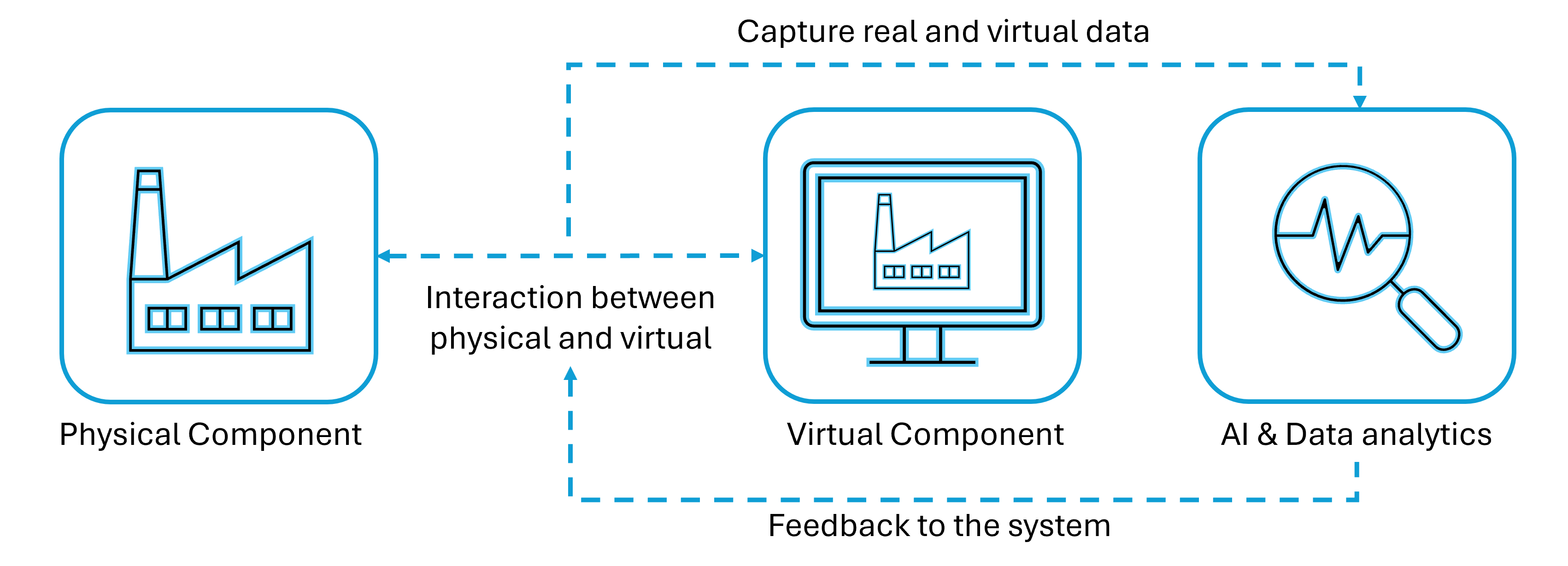
A digital twin is a dynamic, simulation-backed representation of a physical system. It is useful for robotics, instead of testing everything on hardware, many iterations can happen safely in simulation.
It consists of two main components: the physical system and its virtual counterpart. The general workflow of a digital twin is illustrated below:
Here are some advantages of using digital twins:
Managing Complexity
Real systems involve many interacting components that are difficult to reason about analytically. A digital twin combines physics models and data streams to approximate how the system behaves under different conditions, making it easier to plan and optimize.Moving from Reactive to Proactive
When a digital twin continuously monitors a system, it can highlight anomalies and trends early. This supports proactive maintenance instead of waiting for failures, which reduces downtime and cost.Low-Cost Experimentation
New control policies, software updates, or mechanical changes can be evaluated in the twin before they affect the real system. This lowers risk and speeds up development cycles.
Key Components for a Digital Twin Simulation Platform#
To support realistic and scalable digital twins, the underlying simulation platform needs several key capabilities:
General-Purpose Physics Engine
The engine should handle rigid bodies, articulated mechanisms, contacts, and potentially soft materials or fluids. The more accurately it reflects physical behavior, the more reliable the twin becomes.High-Speed Parallelization
Many workflows involve running the same scenario under different conditions—classic in reinforcement learning or parameter sweeps. GPU-accelerated parallel simulation is critical for this.Material Rendering and Visualization
Good visualization is not just cosmetic. It makes debugging easier and helps teams reason about what the robot or system is doing inside the simulated world.Data Integration and Data Generation
A digital twin both consumes and produces data. The platform must be able to ingest sensor or log data and generate synthetic data for analytics or machine learning.
In this blog, we use Genesis as the simulation backend. It is an open-source, GPU-accelerated physics engine designed for robotics and embodied AI, and it can be integrated with AMD hardware through the Vulkan backend.
Tutorial: Controlling a Robot in Genesis Using AMD Ryzen AI MAX#
The following tutorial will guide you on how to use Ryzen AI MAX to control a robot arm on the Genesis platform. Ryzen AI MAX features a unified memory architecture and can allocate up to 96GB of dedicated memory to the GPU, making it an excellent platform for running LLM inference and edge simulations. All content in this tutorial can be executed on Ryzen AI MAX, and complete code samples have been publicly provided.
1. Prerequisites and Initial Setup#
Before working directly with Genesis, it is helpful to have a convenient way to build and run the environment.
The AUP Learning Cloud repository provides a series of pre-configured courses for AMD hardware, using the latest ROCm version to ensure all content runs correctly.
Hardware: AMD Ryzen™ AI Halo device (e.g., AI Max+ 395, AI Max 390)
Environment: Ubuntu 24.04
To get started, clone the repository and install the required dependencies:
git clone https://github.com/AMDResearch/aup-learning-cloud.git
cd aup-learning-cloud/deploy/
sudo ./single-node.sh install
After installation completes, open http://localhost:30890 in your browser. The “Physical Simulation” course in the browser will fully cover the tutorial content presented in this blog.
For users who prefer to install Genesis directly, the official Genesis repository provides detailed instructions. For more information and from-scratch installation instructions, please go to the Genesis repository.
After the installation is ready, you can start a Python session (or Jupyter notebook) and begin building scenes with Genesis.
2. Initialize Genesis Backend#
Genesis needs to be initialized exactly once per process. During this step, it prepares data structures and selects the compute backend. On AMD hardware, the Vulkan backend is recommended to leverage the integrated GPU for rendering.
import genesis as gs
gs.init(backend=gs.vulkan)
3. Create a Simulation Scene#
A scene is the container for the entire simulated world. It holds global physics parameters, camera settings, and the list of entities that will be simulated.
Inside the scene, there are two main components: the simulator and the visualizer, as shown in the figure below.
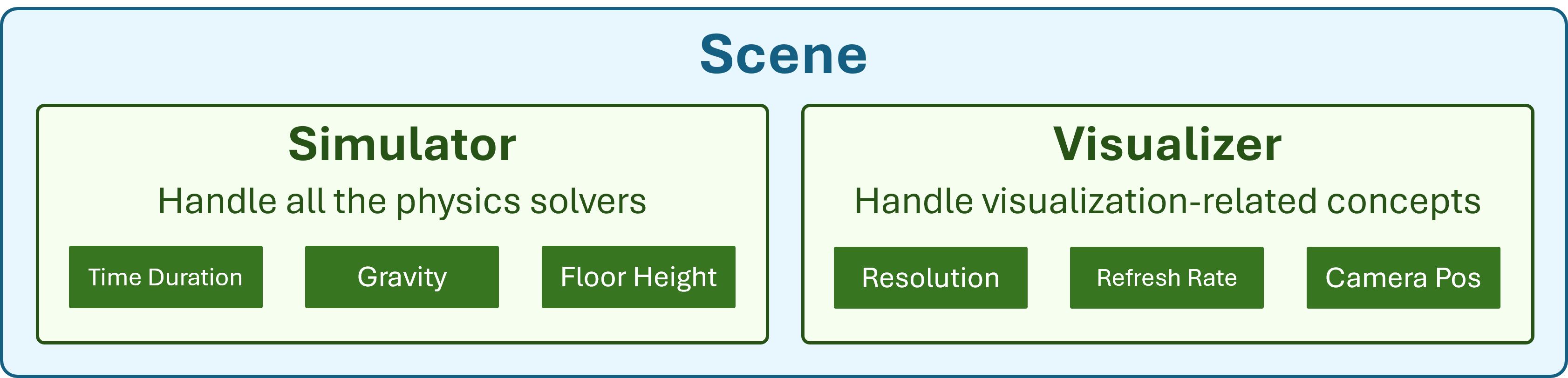
In the example below, the timestep and gravity are specified, and a camera pose is defined. The viewer can be turned off for headless runs.
scene = gs.Scene(
    sim_options=gs.options.SimOptions(
        dt=0.01,
        gravity=(0, 0, -10.0),
    ),
    viewer_options=gs.options.ViewerOptions(
        camera_pos=(3.5, 0.0, 2.5),
        camera_lookat=(0.0, 0.0, 0.5),
        camera_fov=40,
    ),
    show_viewer=False,
)
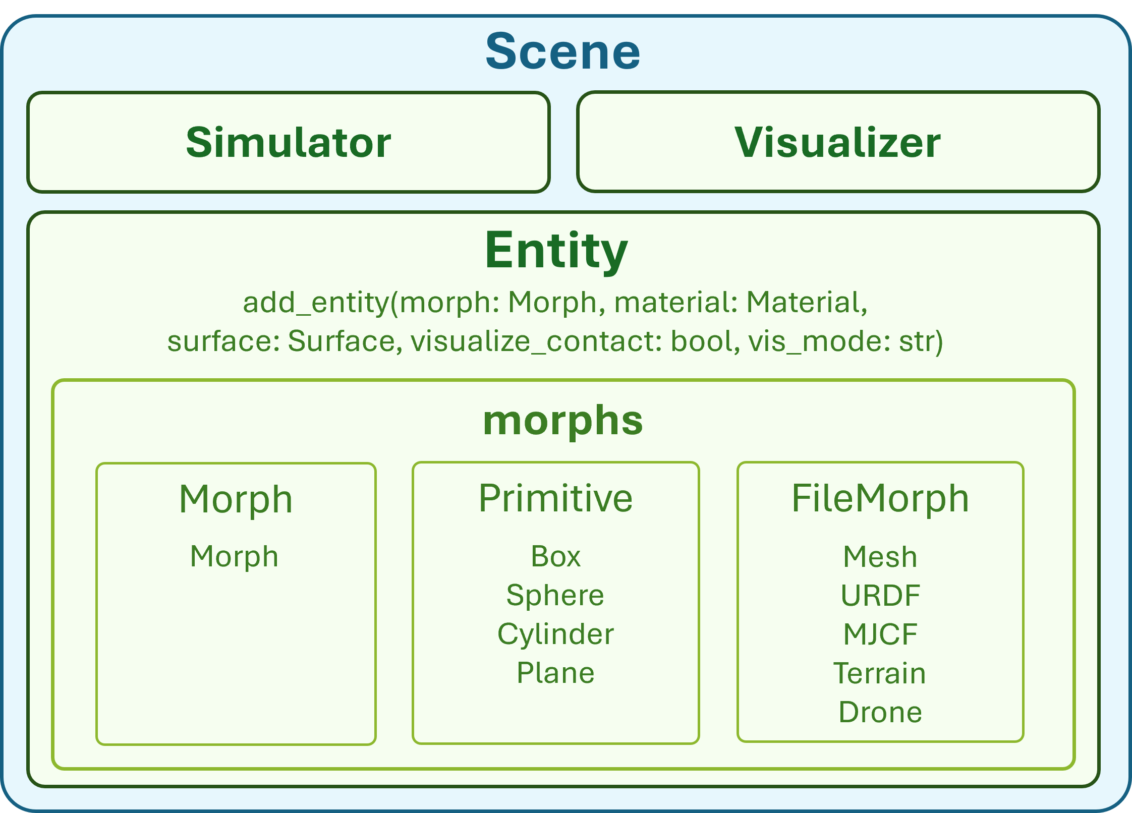
4. Add Entities: Ground and Robot#
Every physical object in Genesis is represented as an entity. You can add different entities to the scene, such as adding a plane, as shown in the figure below.
For a simple robotic setup, a ground plane and a robot arm are enough to get started.
In this tutorial, a Franka Panda arm is loaded from its MJCF file, which encodes its kinematic structure, geometry, and physical properties.
plane = scene.add_entity(gs.morphs.Plane())

franka = scene.add_entity(
    gs.morphs.MJCF(file="xml/franka_emika_panda/panda.xml"),
)
5. Build the Scene#
Before stepping the simulation, Genesis needs to “build” the scene. This is where it inspects the entities, generates optimized GPU kernels, and allocates memory for internal state: positions, velocities, contact data, and controller buffers. After this step, the high-level structure of the scene is fixed.
scene.build()
6. Control Joints and DOFs#
Robot motion is controlled at the DOF (degree of freedom) level. The Franka Panda has 7 arm joints and 2 gripper joints, giving 9 DOFs in total. Genesis stores DOFs in flat arrays on the device, so we first collect their indices to control them efficiently.
jnt_names = [
    'joint1','joint2','joint3','joint4','joint5','joint6','joint7',
    'finger_joint1','finger_joint2'
]

dofs_idx_temp = [franka.get_joint(name).dofs_idx_local for name in jnt_names]
dofs_idx = [idx for sublist in dofs_idx_temp for idx in sublist]
7. Configure PD Controllers#
To produce physically realistic motion, the robot uses PD (Proportional–Derivative) controllers. Each DOF has a stiffness term (Kp), a damping term (Kv), and a torque limit. These values influence how aggressively the joint tries to track its target and how stable the motion feels.
Here, we take the Franka arm as an example:
import numpy as np

franka.set_dofs_kp(
    kp=np.array([4500, 4500, 3500, 3500, 2000, 2000, 2000, 100, 100]),
    dofs_idx_local=dofs_idx,
)

franka.set_dofs_kv(
    kv=np.array([450, 450, 350, 350, 200, 200, 200, 10, 10]),
    dofs_idx_local=dofs_idx,
)

franka.set_dofs_force_range(
    lower=np.array([-87, -87, -87, -87, -12, -12, -12, -100, -100]),
    upper=np.array([ 87,  87,  87,  87,  12,  12,  12,  100,  100]),
    dofs_idx_local=dofs_idx,
)
8. Control Joint Position#
We have two ways to control joint positions: one is direct joint position assignment, and the other is sending control commands through PD.
Direct Joint Position Assignment
When initializing or resetting a scene, it is often convenient to place the robot in a specific configuration immediately. This can be done by directly setting the DOF positions, which overwrites the internal state without going through the physics solver.
franka.set_dofs_position(
    np.array([1, 1, 0, 0, 0, 0, 0, 0.04, 0.04]),
    dofs_idx
)
Sending Control Commands Through PD
For actual motion, commands should go through the PD controllers. This preserves dynamics, respects limits, and results in more realistic behavior. In the example below, the first DOF is driven with a velocity target, while the remaining DOFs are given position targets.
# Position targets for DOFs 1–8
franka.control_dofs_position(
    np.array([0, 0, 0, 0, 0, 0, 0, 0])[0:],  # 8 elements for joints 2–9
    dofs_idx[1:],
)

# Velocity target for the first DOF
franka.control_dofs_velocity(
    np.array([1.0]),   # only for joint1
    dofs_idx[:1],
)
9. Start the Simulation#
The core simulation loop repeatedly advances the scene by one timestep. On each step, Genesis computes controller torques, resolves constraints and contacts, integrates motion, and updates transforms.
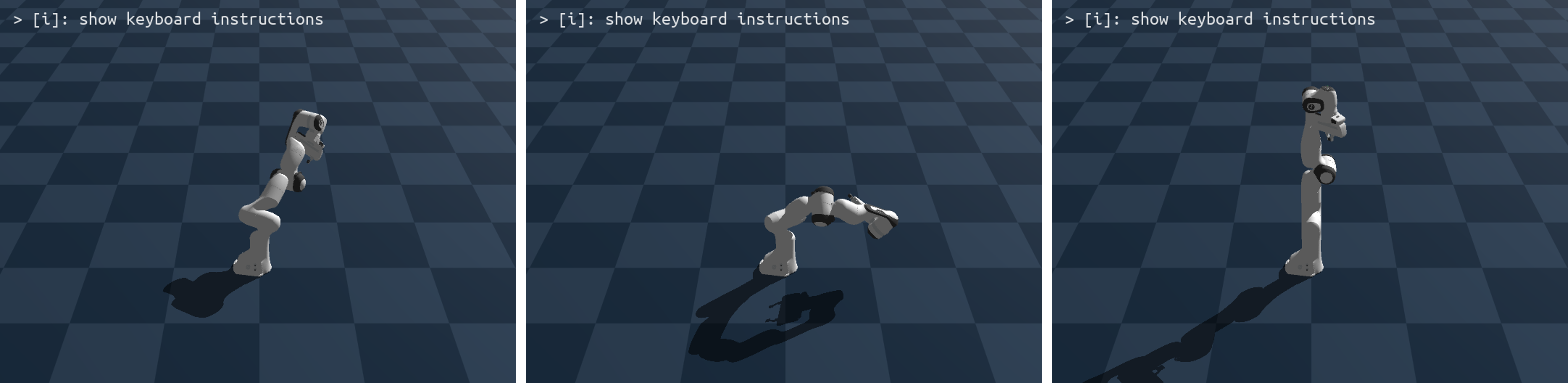
for i in range(120):
    scene.step()
If everything goes smoothly, you will see a robotic arm appear on the screen. A portion of the scene is shown below:
10. Motion Planning With IK#
For tasks like reaching and grasping, it is often easier to specify a target end-effector pose rather than joint angles. Genesis provides inverse kinematics utilities to compute joint configurations that realize a given pose, and these can be turned into trajectories and tracked by the same PD control mechanism.
A typical pipeline looks like this:
Define a target pose for the end-effector.
Use inverse kinematics (IK) to solve for joint angles.
Interpolate between the current and target configurations.
Send the joint targets over time using
control_dofs_position.
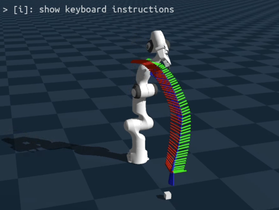
The full implementation depends on the specific task and is usually best placed in a separate notebook or script. When you visualize the motion planning trajectory, you might see a scene like the one below:
11. Parallel Simulation#
Many digital twin and RL workloads benefit from running multiple environments in parallel. Genesis can replicate the scene into a batch of environments during the build stage. Each environment has its own robot state but shares the same GPU kernels and scene structure.
To enable this, the number of environments and the spacing between them are specified when building the scene:
n_envs = 9
scene.build(n_envs=n_envs, env_spacing=(1.0, 1.0))
After this, every state array gains an environment dimension. Control commands and observations can then be handled in a batched way, which is ideal for reinforcement learning or large-scale evaluation.
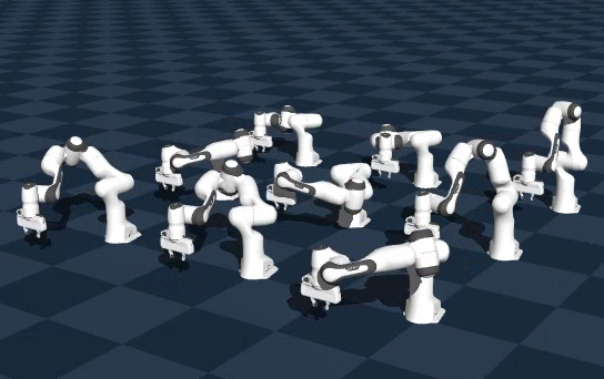
The following figure demonstrates a setup where nine robotic arms are simulated simultaneously:
Summary#
This blog introduced the concept of digital twins, outlined what a capable digital-twin platform needs, and showed how AMD hardware can support this workflow at the edge. Using Genesis on Ryzen AI MAX, we walked through a complete pipeline: initialization, scene creation, robot loading, controller setup, simulation stepping, motion control, and parallel environments.
These pieces form a solid foundation for building more advanced applications such as reinforcement learning, sim-to-real transfer, and large-scale synthetic data generation—all running on AMD hardware with a high-performance, GPU-accelerated simulation stack.
Additional Resources#
AUP Learning Cloud: https://github.com/AMDResearch/aup-learning-cloud
AMD Ryzers Repository: https://github.com/AMDResearch/Ryzers
Genesis Simulation Engine: https://github.com/Genesis-Embodied-AI/Genesis
MJCF Franka Model: https://github.com/facebookresearch/fairo/tree/main/fairo/robots
Acknowledgements#
Thanks to the AMD University Program, AMD Research & Advanced Development teams, and the Genesis Embodied AI community for contributing to open digital-twin research infrastructure.
Disclaimers#
Third-party content is licensed to you directly by the third party that owns the content and is not licensed to you by AMD. ALL LINKED THIRD-PARTY CONTENT IS PROVIDED “AS IS” WITHOUT A WARRANTY OF ANY KIND. USE OF SUCH THIRD-PARTY CONTENT IS DONE AT YOUR SOLE DISCRETION AND UNDER NO CIRCUMSTANCES WILL AMD BE LIABLE TO YOU FOR ANY THIRD-PARTY CONTENT. YOU ASSUME ALL RISK AND ARE SOLELY RESPONSIBLE FOR ANY DAMAGES THAT MAY ARISE FROM YOUR USE OF THIRD-PARTY CONTENT.