Semantic Fencing of Video Streams Using Embedding Splits from Vision Foundation Models

May 15, 2026 by Haani Ahmed, Matthieu Chan Chee, Pier Luigi Dovesi, Max Kiehn.

13 min read. | 3227 total words.

Applications & models

AI/ML, Computer Vision

AI

In this blog, we present a novel approach for semantically splitting vision datasets into training, validation, and test sets. Instead of relying on ad hoc metadata rules or random shuffles, we use embeddings to reason directly about similarity in latent space and construct splits that better reflect true generalization.

We begin by outlining the key concepts and challenges around traditional methods of partitioning datasets, then introduce the key ideas behind our Semantic Fencing data splitting method and finally walk through a step-by-step Jupyter notebook that demonstrates this approach on dashcam sequences from the Zenseact Open Dataset.

The Challenge of Splitting Data

In academic settings, machine learning datasets and benchmarks often include predefined train/validation/test partitions, or one can simply shuffle the data and divide it. In many real-world systems, though, data is not a static table but a continuous, high-volume stream - think of autonomous driving logs for example. These streams exhibit strong temporal, spatial, and semantic correlations, and they are often highly redundant: consecutive frames look nearly identical, the same routes are revisited, and similar scenes are recorded over and over.

In such settings, random splitting is often unreliable. When you shuffle and divide, visually similar samples routinely end up in different partitions: consecutive frames, repeated scenes, or near identical subsequences can appear in both training and evaluation sets. This “semantic leakage” makes metrics less reliable, sometimes inflating them, as the model may end up effectively being tested on data that is only a slight variation of what it has already seen during training. As a result, reported performance may not be representative of how the system will behave on truly novel data, undermining the credibility of model assessment.

To reduce leakage, industry teams often apply domain-specific fencing heuristics that operate on metadata rather than raw content. In autonomous driving, for instance, teams may rely on:

• Geofencing by city or GPS region (illustrated in Figure 1),

• Time-fencing by season or day/night,

• Routefencing by road category.

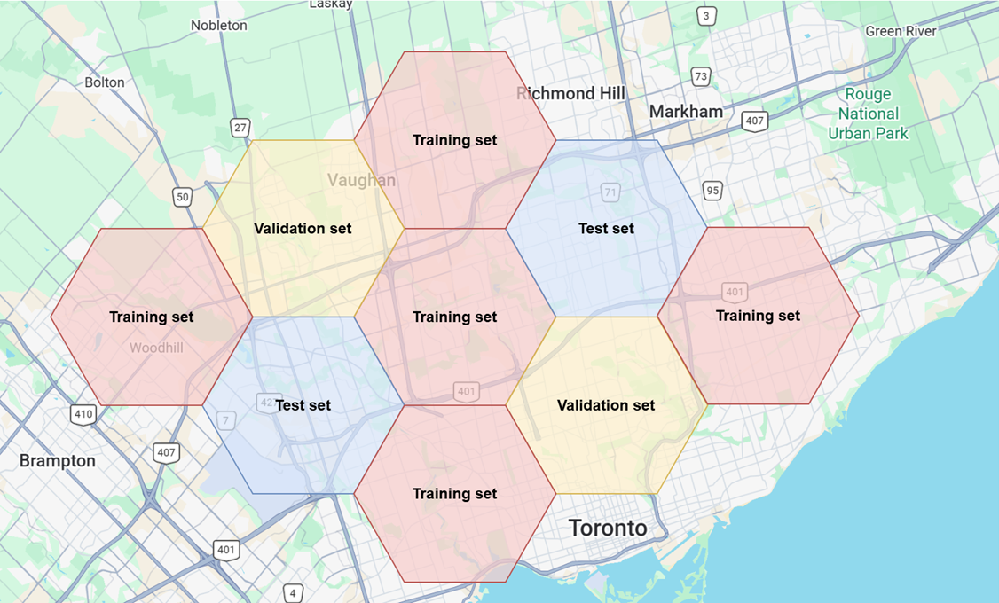
Figure 1. Geofencing can be leveraged to allocate data samples to training, validation or test set based on geolocation

However, such heuristics may not be readily available in other computer vision domains (such as video games, web-scale image classification, retail product imagery, and industrial inspection), as reliable metadata is often missing, noisy, or inconsistent. In the case of simulations and video games, gameplay datasets may lack clean level IDs, map regions, or session markers. Similarly, large web collected vision datasets often have incomplete or incorrect tags, timestamps, or source identifiers. When the metadata cannot be trusted, any splitting strategy that depends on it becomes fragile.

Even when metadata is available, heuristics tend to be highly ad hoc and domain-specific. A fencing scheme based on game maps and missions does not transfer to retail imagery (where you might fence by store, brand, or photoshoot), nor to industrial inspection (where you might fence by production line or batch). Each dataset and application ends up with bespoke rules that require expert judgment to design, maintain, and debug.

Moreover, there is no one-size-fits-all choice of metadata even within a single domain. On the same video game corpus, different teams may want to separate data along very different axes: by map or biome, by difficulty tier, by visual style, by platform, or by game mode. Each of these suggests a different splitting rule, and no single metadata field cleanly captures all of them. In retail or web imagery, splitting by product ID might be appropriate if the goal is to evaluate performance on known catalog items, but disastrous for setups that aim to generalize across brands, styles, or sellers. Teams may compensate by layering multiple heuristics on top of each other, yet still cannot guarantee that semantically near duplicate samples don’t leak across splits.

Because metadata based fencing is task specific, and hard to scale, we need a more principled approach that operates directly on the content. Hence, we turn to a more general paradigm of Semantic Fencing: splitting data according to its latent space characteristics, using embeddings to capture and separate regions of semantic similarity rather than relying solely on handcrafted metadata heuristics.

From Visual Meaning to Latent Space Structure

Modern vision foundation models, such as CLIP, DINO, and their successors, are trained on massive, diverse image (and image text) corpora, allowing them to learn rich, general-purpose visual representations. Instead of focusing on a narrow task like classifying a fixed set of labels, these models learn to encode high-level “visual meaning”: scene layout, object categories, textures, viewpoints, and even stylistic cues.

They do this by mapping each image to a high-dimensional embedding vector whose geometry reflects semantic similarity. Images that are conceptually related (such as frames from the same game map, different angles of the same scene, or visually similar environments) are mapped to nearby points in this latent space, while semantically different images end up far apart. Because these embeddings are learned from broad and varied training data, they tend to be robust to nuisance factors like minor viewpoint changes, small occlusions, or slight lighting shifts, making them well suited for reasoning about visual similarity at scale.

When we apply these models to sequential data such as videos or gameplay logs, a long clip becomes a “trajectory” of points moving through latent space, as shown in Figure 2. As the camera moves, the player transitions between areas, or the scene evolves, that embedding trajectory shifts accordingly. This lets us reason not just about individual frames, but about how visual semantics evolve over time, and, crucially, carve this trajectory into coherent segments reflecting the true structure of the data, instead of relying on ad hoc domain-specific metadata rules.

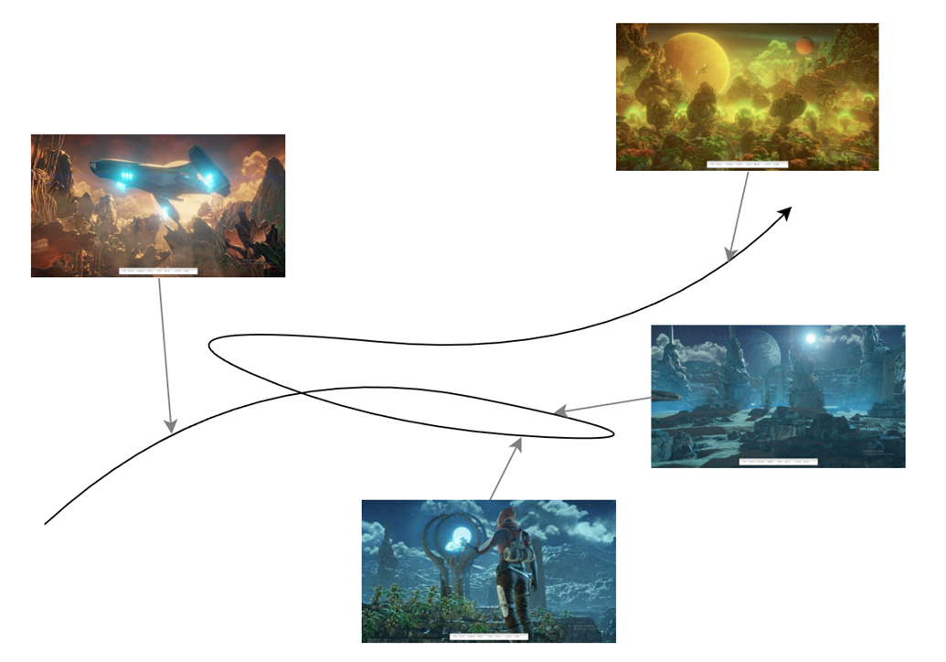
Figure 2. A trajectory of points from a visual data stream in embedding space

The trajectory can be partitioned into training, validation, and test sets by defining bounded semantic regions and assigning points according to their location within those regions. As shown in Figure 3, we represent these regions as nested spheres:

• Points within the innermost spheres are assigned to the validation set,

• Points between the inner and outer spheres are designated for the test set, and

• Points outside all spheres are allocated to the training set.

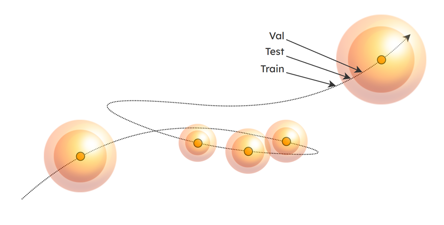
Figure 3. Semantic fencing of regions in latent space to split training, validation, and test sets

This strategy allows us to move away from domain-dependent heuristics and directly leverage the latent-space representation of images to establish consistent and semantically grounded dataset splits.

This, however, also leads to several important questions: Where should these regions be placed? How large should they be? And how does the system behave as new data streams are ingested? With the overall concept established, we now delve step-by-step into the technical considerations that guide these choices.

Detailed Mechanics and Walkthrough

We have implemented this method as BubbleFence, a modular pipeline that ingests trajectories of visual data over time and automatically curates semantically meaningful train/validation/test splits using bounded semantic regions (“bubbles”). Each bubble is centered on an anchor, a point in the embedding space that defines where the region is placed. Anchors are selected from the data itself, and each one governs a bubble whose radius determines how many nearby points are captured for evaluation. BubbleFence can be used in three ways: as a CLI (python run_bubblefence.py --folder ... for a single folder, or --batch batch.yaml to process many folders in sequence), programmatically via run_folder() / run_batch() in Python, or declaratively through a batch YAML that lists input folders and desired visualizations. The entire pipeline is configured through a single YAML file (bubblefence_config.yaml).

Below, we walk through the method step by step on dashcam sequences from the Zenseact Open Dataset (ZOD) Drives subset.

The table below maps each algorithmic concept to the config key you would tweak and the underlying class you can import directly if you want to experiment at a lower level.

Concept	Config section	Key params	Class
Embedding	foundation_models	primary_model	FoundationModelProcessor
Deduplication	deduplication	similarity_threshold	handled inside BubbleFencePipeline
Density-adaptive warping	density_transformation	enabled, method	DensityAnalyzer
QMC anchor placement	anchor_placement	method, qmc_sequence, snap_strategy	AnchorPlacer
Adaptive bubble radii	hypersphere	radius_computation, adaptive_method, base_radius_percentile	AnchorPlacer
Nested val/test shells	nested_shells	enabled, validation_ratio	AnchorPlacer
Split targets	dataset_splits	train_ratio, eval_ratio, min_eval_per_batch	BubbleFencePipeline
Streaming persistence	streaming	persistent_anchors, anchor_persistence_path	BubbleFencePipeline

Configuration

The pipeline is configured through a single YAML file (bubblefence_config.yaml). We load it and inspect the key parameters:

from bubblefence import load_config, run_batch

config = load_config("config/bubblefence_config.yaml")

The key parameters are:

Encoder:            openai/clip-vit-base-patch32
Dedup threshold:    0.9999
Anchor placement:   QMC (sobol)
Snap strategy:      lid_weighted
Radius:             adaptive (LID)
Nested shells:      True (val ratio 0.5)
Target split:       0.8 train / 0.2 eval

Note that the deduplication threshold is set to 0.9999 here to preserve near-identical frames for cleaner trajectory visualizations. In practice, a lower threshold (for example, 0.98) provides more aggressive deduplication.

When a folder of images is ingested, the pipeline runs the following steps in order. Each step maps to a section of the config YAML (shown in the table above), so every aspect of the pipeline’s behavior can be tuned without changing code.

1. Embedding and Deduplication (foundation_models, deduplication): Each frame is passed through a frozen vision encoder (such as CLIP) to produce an embedding vector. Near-duplicate frames are then removed based on a cosine similarity threshold, thinning the trajectory while preserving its semantic structure.

2. QMC Anchor Placement (anchor_placement): Quasi-Monte Carlo sequences (Sobol or Halton) propose candidate anchor positions that cover the embedding space uniformly. Each candidate is snapped to a nearby data point using a LID-weighted strategy that biases placement toward denser, more representative regions. Local Intrinsic Dimensionality (LID) is an estimate of the effective dimensionality of the data manifold around a point: low LID indicates a locally flat, dense region while high LID indicates complex, sparse geometry. By weighting snap targets by inverse LID, anchors are drawn toward well-populated areas of the space. When class_aware mode is enabled, the pipeline maintains per-class eval targets and proposes anchors within each class’s embedding subspace, scheduling rare classes first to ensure balanced representation.

3. Adaptive Bubble Construction (hypersphere): Around each anchor, a bubble (bounded semantic region) is constructed with a radius scaled by the local LID: high LID (sparse, complex regions) yields a larger radius to capture enough points, while low LID (dense, flat regions) yields a smaller radius to avoid over-capturing. The radius is clamped between configurable min_radius and max_radius bounds, and further shrunk if the bubble would collide with existing train points or capture more evaluation points than the target ratio allows. Anchors are proposed in a closed loop until the eval quota is met: the pipeline over-proposes candidates, then accepts them one by one, checking the remaining eval deficit after each, and stops as soon as the target is filled.

4. Nested Evaluation Shells (nested_shells): Each bubble is subdivided into two concentric regions: an inner shell (closest to the anchor center) and an outer shell (the ring between the inner boundary and the bubble edge). One shell is assigned to validation and the other to test, so that the two eval splits occupy different distances from the anchor center. The shell_configuration parameter controls this mapping: "inner_val" places validation in the inner shell and test in the outer, "inner_test" does the reverse, and "random" (the default) flips a coin per anchor so that neither split is systematically closer to or farther from anchor centers. Points outside all bubbles are assigned to training.

5. Density-Adaptive Warping (optional) (density_transformation): When enabled, LID is estimated across the embedding space and a warp is applied that expands dense regions and contracts sparse ones, normalizing the effective point density so that downstream bubble sizing behaves consistently regardless of how clustered the data is. This step is disabled by default and is not used in the demo below.

6. Streaming Persistence (streaming): After each ingestion run, all anchors, embeddings, and assignments are persisted to disk. On subsequent runs, existing bubbles are loaded and incoming frames that fall inside them are assigned automatically, with new anchors placed only if the eval ratio needs topping up.

Round 1: Initial Data Ingestion

All experiments were run on an AMD MI325X GPU. Running on CPU is also supported.

A batch YAML (config/zod_round1.yaml) defines the folders to process, the output directory, and the visualizations to generate:

# config/zod_round1.yaml
folders:
  - zod_data/drives/000000/camera_front_blur
  - zod_data/drives/000004/camera_front_blur

output_dir: zod_notebook_exp
bf_config: config/bubblefence_config.yaml

visualizations:
  - type: standalone
    save: tsne_traj_circles_thumbs.png
    show_trajectories: true
    show_radius_circles: true
    show_anchor_thumbnails: true
    reduction_method: TSNE

  - type: stats

  - type: summary
    save: tsne_summary.png
    show_heatmap: true
    reduction_method: TSNE

A single run_batch() call processes all folders, generates visualizations, and prints summary statistics:

run_batch("config/zod_round1.yaml")

The pipeline processes both folders, places anchors, assigns splits, and reports the following statistics:

Total data points: 4,808
Runs: 2

       Train:  3,825 (79.6%)
  Validation:    398 (8.3%)
        Test:    585 (12.2%)

Anchors: 5
  Mean radius: 0.0447
  Std radius:  0.0056
  Min/Max:     0.0360 / 0.0516
  Mean points/anchor: 196.6

To visualize the high-dimensional embedding space, we run t-SNE on the 512-dimensional model embeddings of all data points, projecting them down to two dimensions. Projecting the true hypersphere boundaries into t-SNE space would be intractable, and the non-linear distortions of t-SNE mean that the projected boundaries would not necessarily contain all of a bubble’s assigned points anyway. Instead, for each anchor, we compute the mean Euclidean distance in the 2D t-SNE space from the projected anchor to all data points assigned to that bubble, and draw a circle with that average radius. To visualize trajectories, the temporally ordered points from each run are connected using arc-length-parameterized cubic B-splines (via scipy.interpolate.splprep), producing smooth curves that follow the embedding path through the projected space.

Note that bubbles may overlap in the original embedding space, which is permitted as long as each newly proposed bubble captures a minimum number of new evaluation points. In the t-SNE projection, the non-linear distortions can exaggerate this effect, sometimes making it appear as though one bubble is entirely contained within another when in fact they only partially overlap in the high-dimensional space.

The trajectory plot (Figure 4) shows this t-SNE projection with bubble radius circles and auto-selected anchor thumbnails. The thumbnails show the representative image closest to each anchor center, giving a visual sense of what each bubble “contains”. The two drives (000000 in blue, 000004 in orange) occupy distinct regions of the embedding space, with 5 anchors placed across both trajectories. The anchor thumbnails reveal the visual content each bubble captures, highway scenes, overpasses, and wet road conditions each cluster in its own neighborhood:

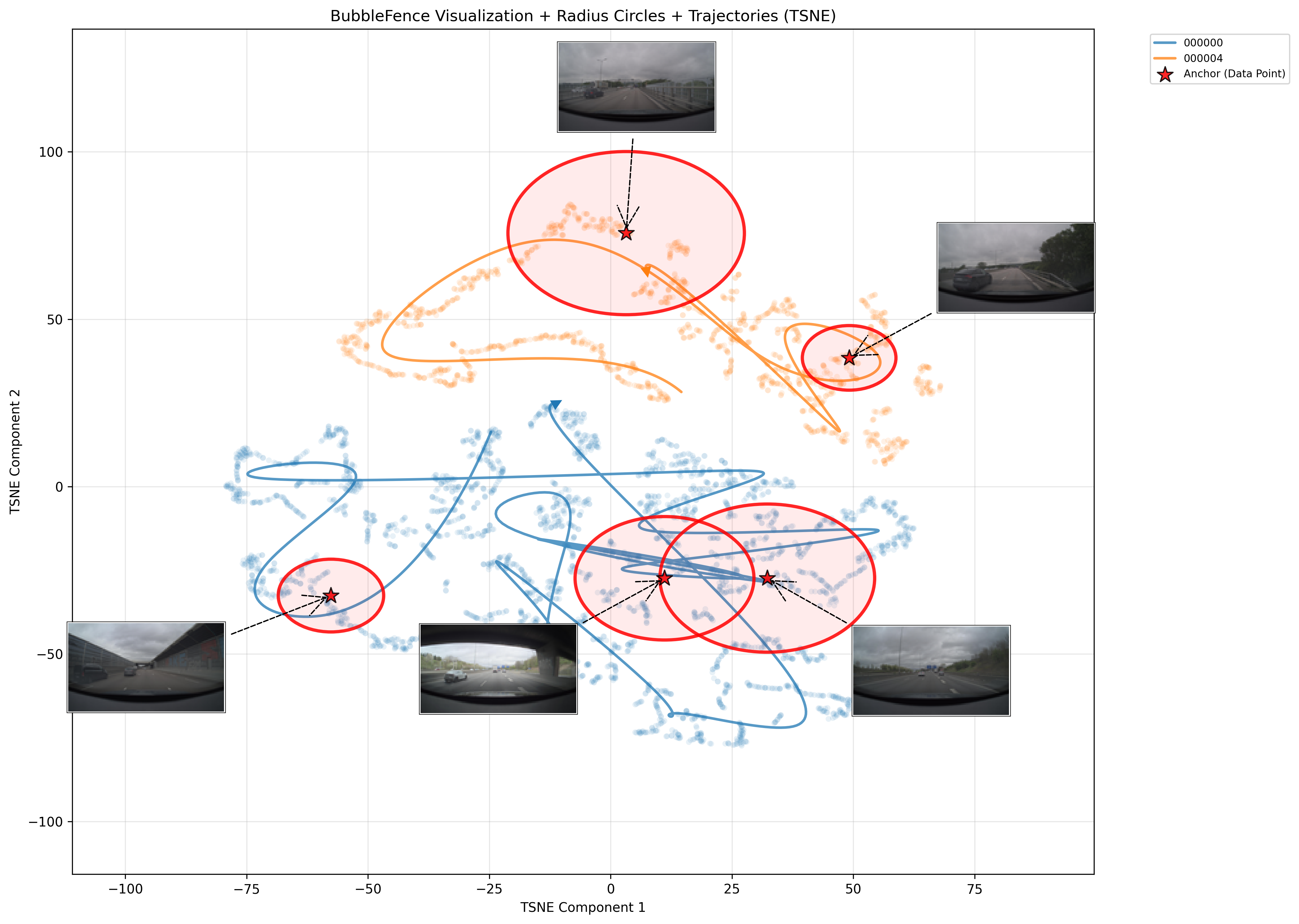
Figure 4. Round 1 trajectory plot showing embedding trajectories with bubble regions and anchor thumbnails. Circles show the average bubble radius in the projected space.

The 2-panel summary (Figure 5) confirms the split structure. The left panel colors each point by its assigned split (blue = train, orange = validation, green = test), showing that eval points are concentrated inside the bubble regions while the bulk of the data remains as training. The right panel overlays an anchor bubble heatmap, highlighting the density of coverage around each anchor center:

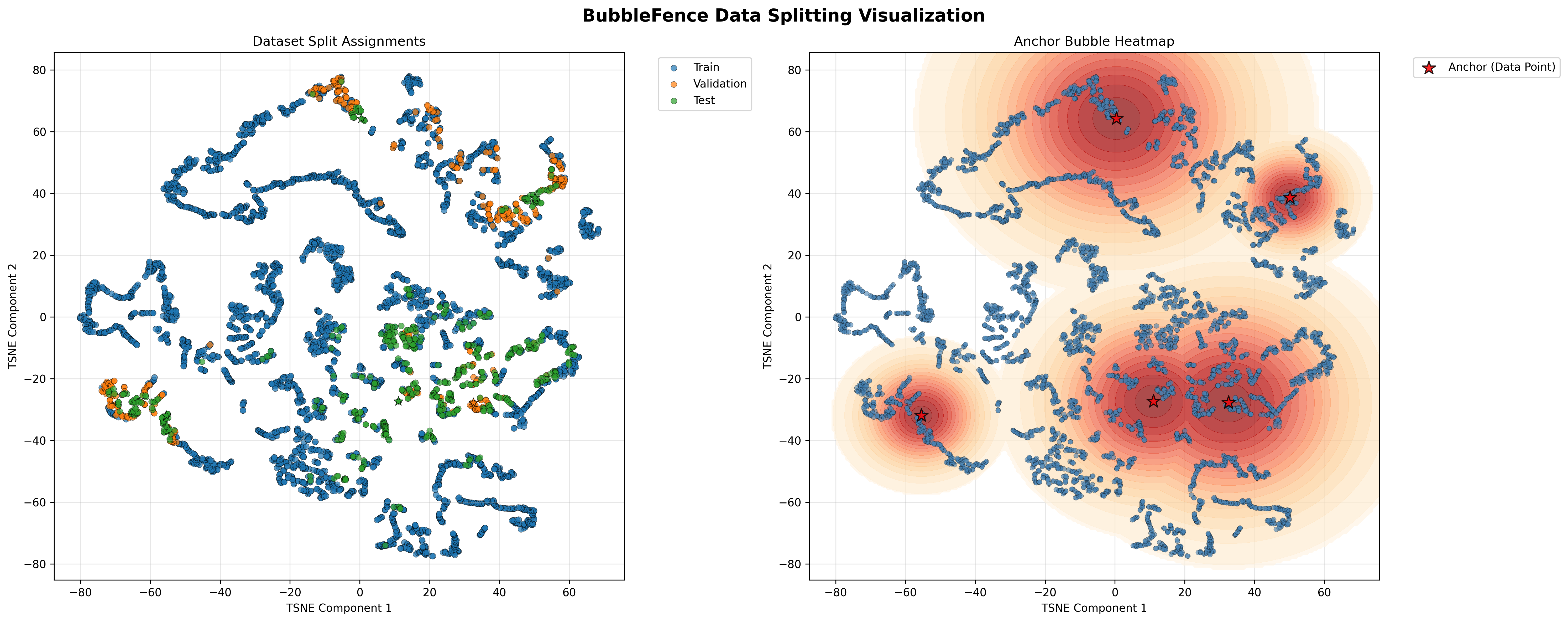
Figure 5. Round 1 summary showing split assignments and anchor bubble heatmap

Round 2: Incremental Dataset Growth with Persistent Anchors

BubbleFence is designed for continual curation: new data streams in over time and the split structure grows with it. Anchors and embeddings from Round 1 are loaded from disk automatically. Incoming frames that fall inside existing bubbles are assigned instantly; new anchors are only placed if the eval ratio needs topping up. This is the streaming persistence mechanism at work.

A second batch YAML adds three more drives, pointing at the same output directory so state is picked up automatically:

run_batch("config/zod_round2.yaml")

With the three new drives ingested alongside the two from Round 1, the updated statistics are:

Total data points: 10,758
Runs: 5

       Train:  8,596 (79.9%)
  Validation:  1,118 (10.4%)
        Test:  1,044 (9.7%)

Anchors: 19
  Mean radius: 0.0561
  Std radius:  0.0134
  Min/Max:     0.0310 / 0.0785
  Mean points/anchor: 113.8

The split ratios closely match the configured 80/20 train/eval target, with the eval portion further divided into validation and test by the nested shell structure. The updated trajectory (Figure 6) and summary (Figure 7) plots now show all five drives:

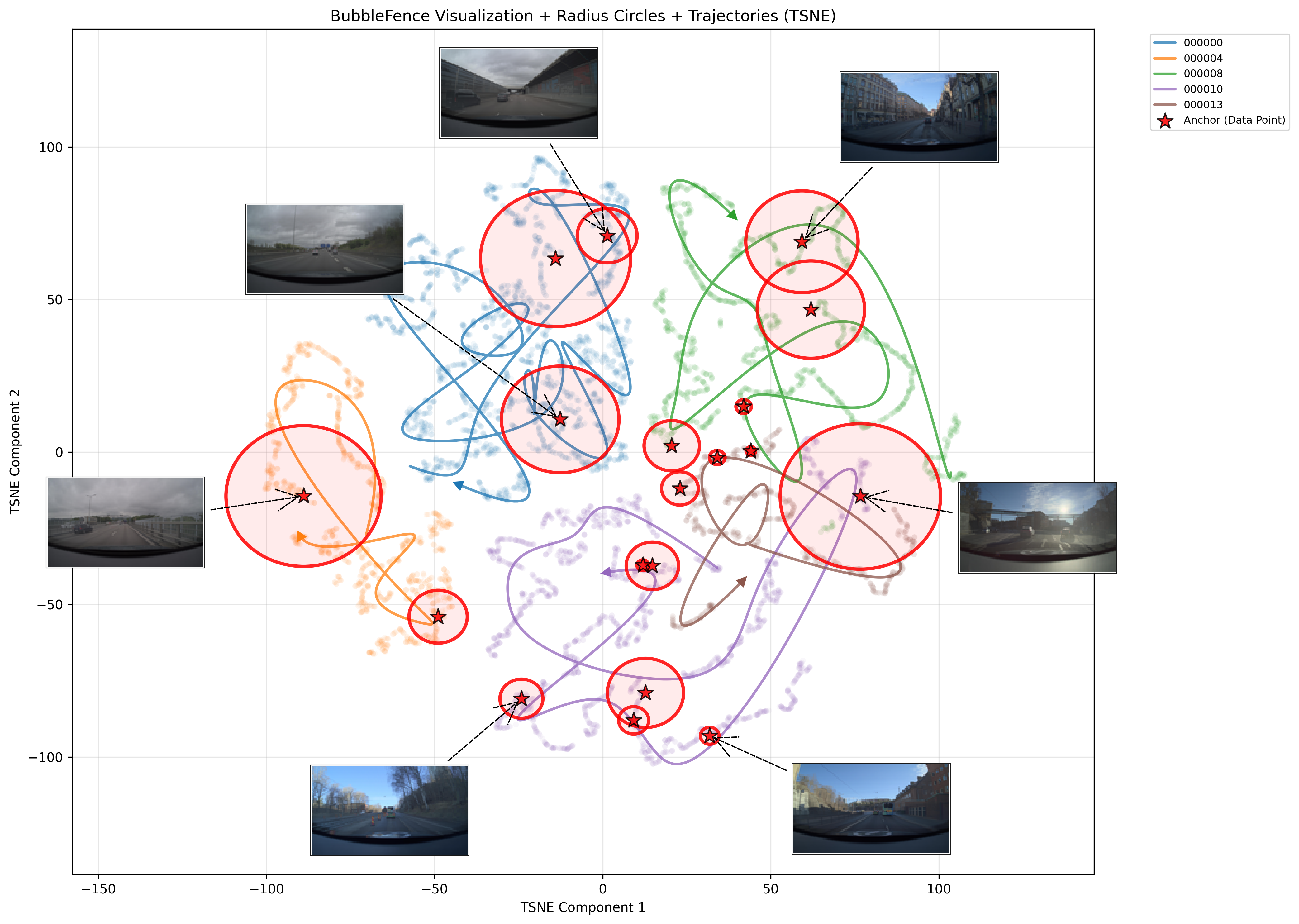
Figure 6. Round 2 trajectory plot after ingesting five drives, showing how new trajectories integrate with existing bubble regions. Circles show the average bubble radius in the projected space.

Note how the t-SNE projection organizes the data by visual content: trajectories on the left side of the plot correspond to highway driving scenes, while those on the right side correspond to urban areas. This separation emerges naturally from the embedding space and illustrates the kind of semantic structure that BubbleFence exploits for splitting.

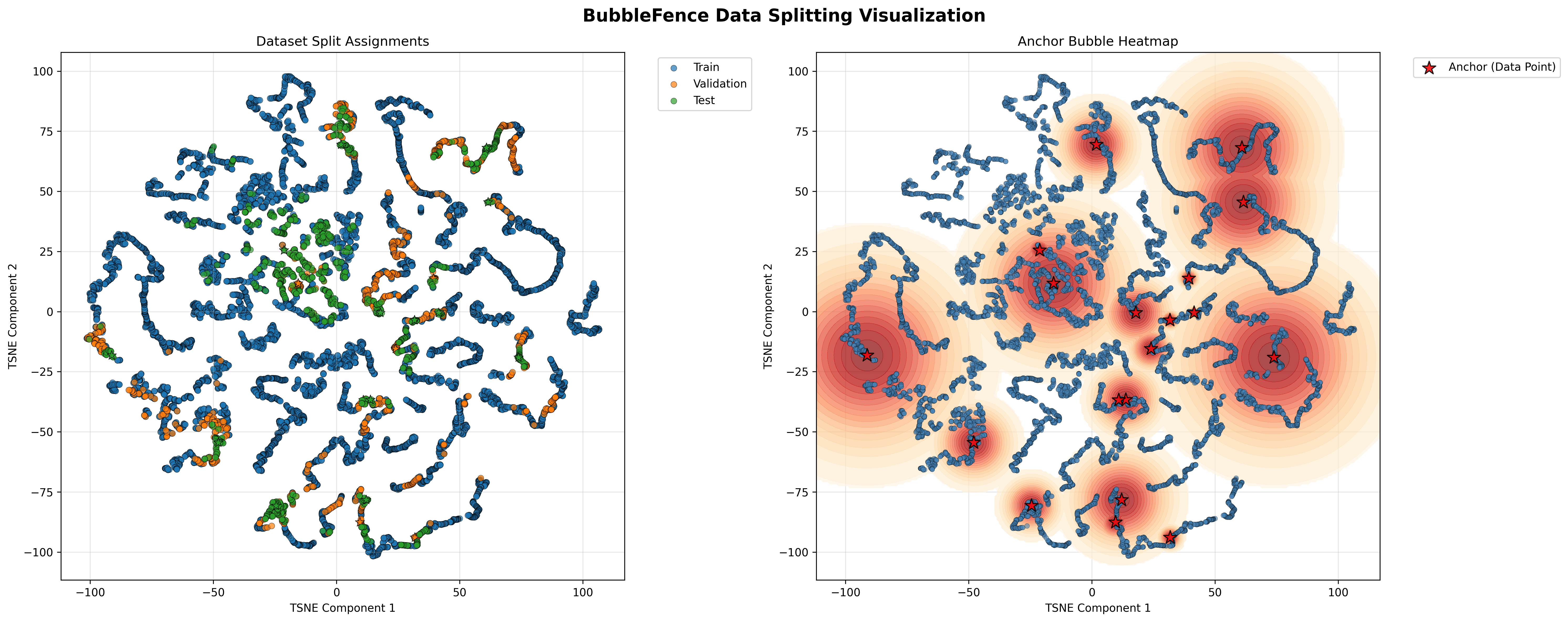
Figure 7. Round 2 summary showing updated split assignments and anchor bubble heatmap across all five drives

Notice how the bubbles from Round 1 persist and automatically capture semantically similar frames from the new drives, while new anchors are added only where needed to maintain the target eval ratio. This demonstrates the key advantage of BubbleFence: the split structure is stable and grows incrementally with new data, without requiring reprocessing of previously ingested content.

3D Embedding Visualization

The t-SNE projections shown above reduce the high-dimensional embedding space to two dimensions for clarity, but this inevitably loses some structural information. To better appreciate the spatial relationships between trajectories and bubble regions, we can also render the t-SNE projection in three dimensions. The interactive 3D view below allows rotation and zooming, revealing cluster separations and bubble placements that may overlap or appear ambiguous in the 2D projection.

Figure 8. Interactive 3D t-SNE projection of embedding trajectories and bubble regions

Applying BubbleFence to Other Domains

While the walkthrough above focuses on autonomous driving data, BubbleFence is designed to be domain-agnostic. To illustrate this, we apply the same pipeline to a completely different visual domain: video games. Specifically, we run BubbleFence on image frames extracted from a random selection of contractor demonstration videos released as part of OpenAI’s Video PreTraining (VPT) project (code and data), with no changes to the pipeline configuration beyond pointing it at the new data.

Total data points: 12,932
Runs: 4

       Train: 10,226 (79.1%)
  Validation:  1,997 (15.4%)
        Test:    709 (5.5%)

Anchors: 31
  Mean radius: 0.0314
  Std radius:  0.0108
  Min/Max:     0.0148 / 0.0581
  Mean points/anchor: 87.3

The trajectory plot (Figure 9) reveals how the embedding space organizes Minecraft gameplay by visual context. Distinct clusters emerge corresponding to different terrain types and environments: outdoor scenes with grass and trees occupy one region, underground cave and mine areas cluster separately, and indoor or structure-based scenes (wooden interiors, crafting areas) form their own neighborhoods. The anchor thumbnails confirm this semantic grouping, with each bubble capturing a visually coherent set of frames. Compared to the autonomous driving results, the bubbles here tend to have smaller radii (mean 0.0314 versus 0.0561), reflecting the tighter, more discrete clusters that arise from Minecraft’s distinct biome and environment types rather than the smoother, continuous transitions of real-world driving trajectories.

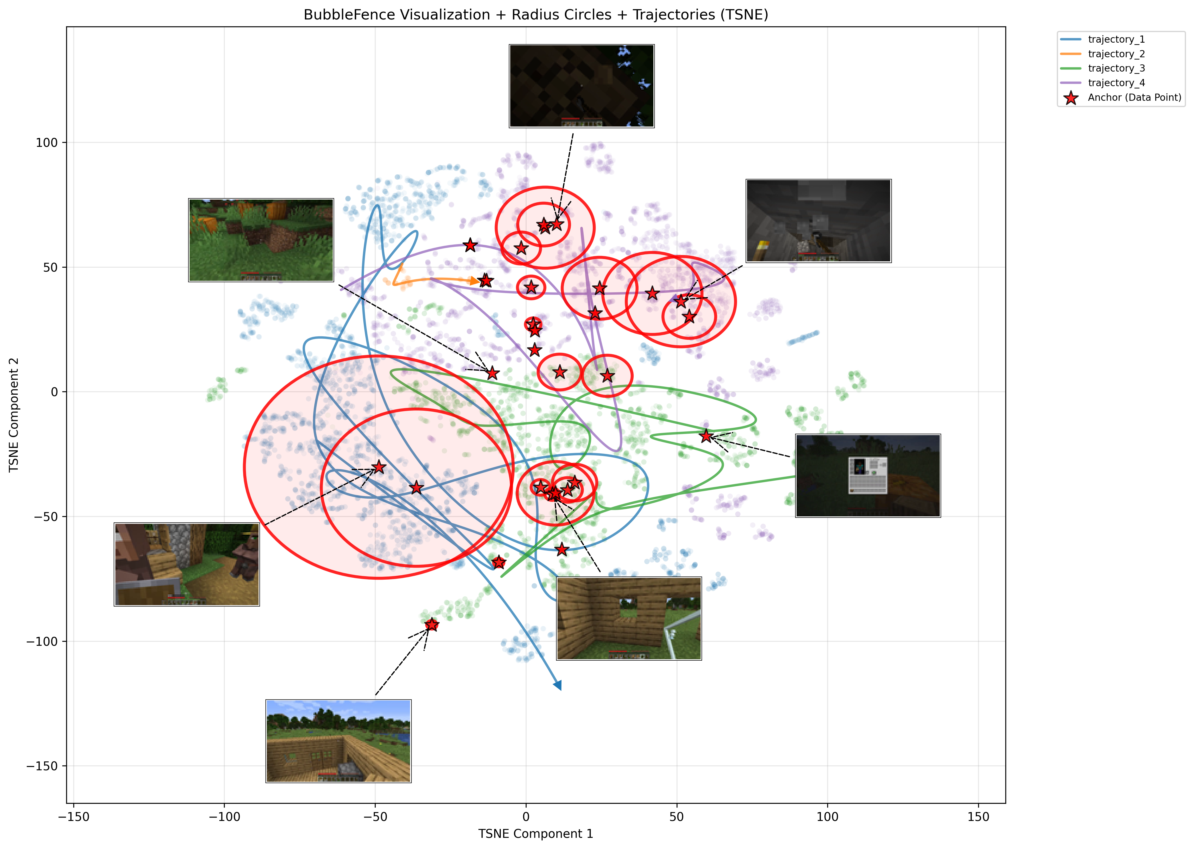
Figure 9. Minecraft gameplay trajectory plot showing embedding trajectories with bubble regions and anchor thumbnails across four gameplay videos. Circles show the average bubble radius in the projected space.

The summary plot (Figure 10) shows the split assignments and anchor bubble heatmap. The left panel highlights how eval points (orange and green) are concentrated within the bubble regions while the majority of frames remain as training data (blue), maintaining the target 80/20 split ratio. The right panel’s heatmap reveals that anchor coverage is denser in the lower-left region of the projection, where several gameplay sessions overlap in visually similar outdoor and terrain-exploration scenes, while more isolated clusters (such as indoor and underground environments) receive fewer but smaller bubbles.

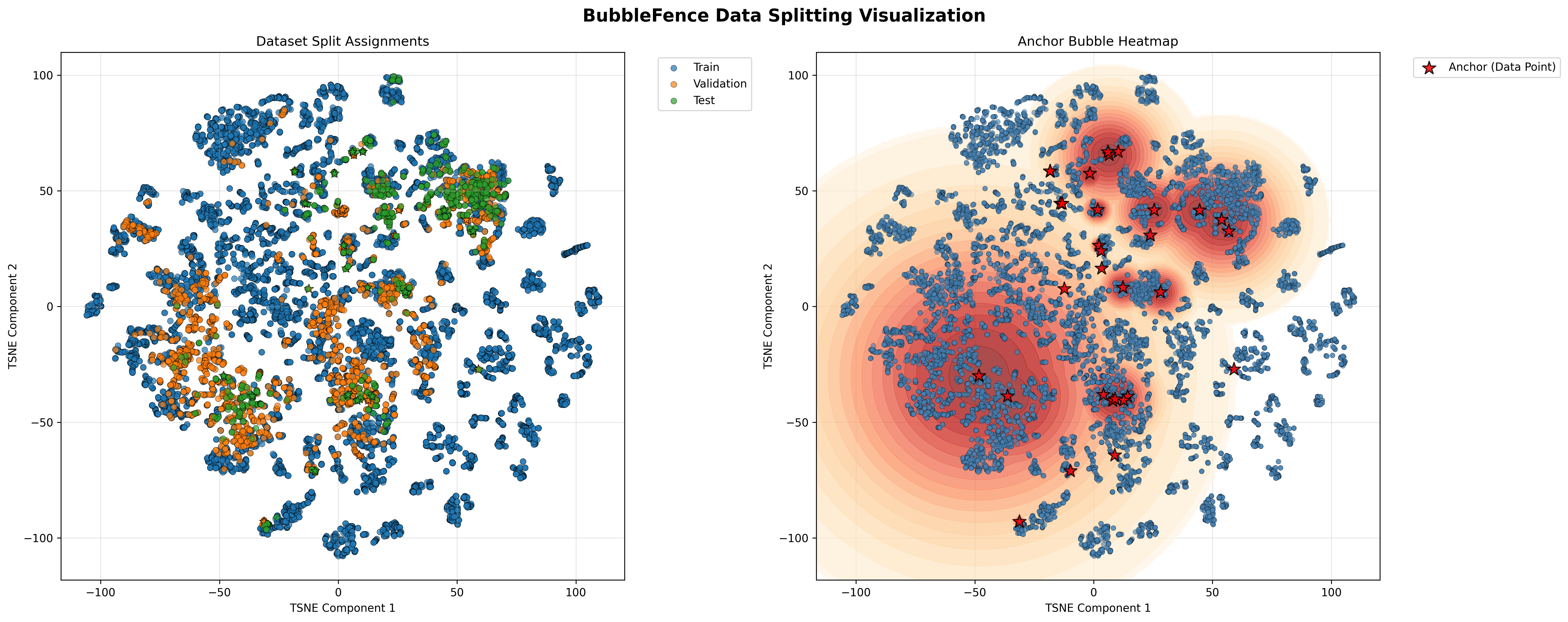
Figure 10. Minecraft gameplay summary showing split assignments and anchor bubble heatmap

The fact that BubbleFence produces coherent, semantically grounded splits on Minecraft gameplay data, without any domain-specific tuning, demonstrates the generality of the approach. The same pipeline that split dashcam trajectories while taking into consideration factors such as road type and driving conditions here splits gameplay frames by terrain, lighting, and environment type, relying entirely on the foundation model’s learned representations.

Limitations and Future Work

The quality of the splits depends on the foundation model’s ability to capture meaningful semantic similarity for the domain at hand. A model trained primarily on natural images may not produce useful embeddings for highly specialized content such as medical scans or synthetic data, which would require a domain-appropriate encoder. Additionally, if the data is uniformly distributed in embedding space with no natural clusters or density variation, the bubble placement has less semantic structure to exploit and the resulting splits may offer limited advantage over random partitioning. Finally, while BubbleFence adds modest computational overhead compared to a simple random shuffle, the embedding step requires a forward pass through a vision model for every frame, which makes GPU acceleration effectively a requirement for large-scale deployments.

Summary

This blog outlined the practical difficulties of splitting real-world data, as traditional heuristics based on geography or time struggle to capture semantic structure and often fail to prevent leakage. By moving the split logic into the embedding space, we gain a principled framework for reducing semantic leakage, improving evaluation reliability over time, adapting as new content appears, and supporting long-term, continually evolving data ingestion engines.

Although we illustrated the idea here in the autonomous driving and gaming contexts, the technique is generalizable across various other domains, including robotics, simulation environments, and any setting that produces high-volume visual data. As our approach is in its early stages of development, we aim to further experiment and refine it in future work.

Notes: This approach was proposed as part of patent application US19465844.

Acknowledgement

This work has been supported by the EuroHPC JU project “MINERVA” (GA No. 101182737).

Disclaimers

Third-party content is licensed to you directly by the third party that owns the content and is not licensed to you by AMD. ALL LINKED THIRD-PARTY CONTENT IS PROVIDED “AS IS” WITHOUT A WARRANTY OF ANY KIND. USE OF SUCH THIRD-PARTY CONTENT IS DONE AT YOUR SOLE DISCRETION AND UNDER NO CIRCUMSTANCES WILL AMD BE LIABLE TO YOU FOR ANY THIRD-PARTY CONTENT. YOU ASSUME ALL RISK AND ARE SOLELY RESPONSIBLE FOR ANY DAMAGES THAT MAY ARISE FROM YOUR USE OF THIRD-PARTY CONTENT.

3DMark is a registered trademark of UL Solutions. Screenshots are reproduced for illustrative benchmarking and technical discussion purposes only. UL Solutions does not sponsor, endorse, certify, or validate this publication or the products, methodologies, or conclusions discussed herein.

The demo in this blog uses data from the Zenseact Open Dataset (ZOD), which is the property of Zenseact AB (© 2022 Zenseact AB) and is licensed under CC BY-SA 4.0. For this dataset, Zenseact AB has taken all reasonable measures to remove all personally identifiable information, including faces and license plates. To the extent that you like to request removal of specific images from the dataset, please contact privacy@zenseact.com. The ZOD development kit is licensed under the MIT License.

The Minecraft gameplay frames used in this blog were extracted from contractor demonstration videos released by OpenAI as part of the Video PreTraining (VPT) project. The VPT repository is licensed under the MIT License with respect to the code. Minecraft is the intellectual property of Microsoft. AMD does not purport to license, sublicense, or otherwise transfer any intellectual property rights with respect to Minecraft, and such visuals are included solely for illustrative and research purposes.