High-Resolution Weather Forecasting with StormCast on AMD Instinct GPU Accelerators#

The traditional approach to numerical weather prediction is based on propagating a known atmospheric state forward in time in short steps using systems of partial differential equations directly obtained from physical considerations. A new approach is to use machine learning methods to directly proceed to a later state in one large step, typically moving forward multiple hours in a single jump.
The newer machine learning based approach is currently evolving rapidly, and has already achieved parity with, or supremacy over, the best traditional methods over a number of metrics. One especially interesting capability of these new methods is the ability to generate high-resolution, local forecasts of strongly convective phenomena such as thunderstorms using only a limited amount of computational resources.
In this blog entry, we will first briefly outline the complexities of weather prediction on different scales, and point out the elements that have proven particularly difficult for traditional methods. We will then discuss how machine learning based approaches can successfully sidestep some of these difficulties.
Next, we will demonstrate how you can use AMD Instinct GPU accelerators to run a particular high-resolution, convection-emulating AI model called StormCast. We will show how to install the model and run forecasts. We will also demonstrate how you can create plots comparing your results to the state of the art analysis results produced by NOAA, the National Oceanic and Atmospheric Administration, the main weather forecasting agency of the United States.
Weather forecasting at different scales#
Meteorology uses a number of spatial and temporal scales defined roughly by what processes typically occur at these scales and what drives them. Typical definitions (see e.g. [1]) define a spatial micro-, meso- and macro-scale, and a temporal micro-, meso-, synoptic and climatological scale. While spatial and temporal micro and meso-scales roughly correspond, the spatial macro-scale overlaps with both synoptic and climatological temporal scales.
Micro-scale#
At one extreme, the spatial and temporal micro-scale represents spatial extents of roughly one kilometer or less, corresponding also to events with a timescale of around one hour or less. At these scales, atmospheric phenomena are characterized by timescales defined by the frequency of atmospheric gravity waves, and the local turbulent advective time scale.
Micro-scale covers phenomena ranging from tornadoes at the scales of a kilometer and an hour down to turbulence at the scales of meters and seconds. These phenomena are highly local and difficult to predict, as a prediction would require knowledge of the state of the local atmosphere at a high resolution, and the phenomena themselves are ephemeral in nature.
Macro-scale#
At the other extreme we have the synoptic and climatological timescales from one day to months and years, and in spatial extent from around 2000 km upwards, that is, the spatial macro-scale. At these scales the effects of the Earth’s rotation become important, and the relevant timescales are related to the variation of Earth’s rotational speed with latitude and the Rossby radius of deformation, as well as the inverse of Earth’s rotational frequency. The macro-scale atmospheric dynamics, especially in the upper atmosphere, are dominated by the balance between pressure gradient forces and the Coriolis force, resulting in what is called geostrophic flows.
Phenomena at the macro-scale range from tropical cyclones and weather fronts to planetary atmospheric tides. Predicting atmospheric evolution at these scales has a long history, since various simplifying approximations such as the aforementioned geostrophic approximation are possible. However, numerical weather prediction at these planetary scales has traditionally required implementing a number of subgrid models. These are required to represent physical interactions and phenomena that occur at smaller scales than the computational grid can resolve. This can be the case for e.g. clouds, turbulence, orographic effects and importantly for us, convection (see e.g. [2]).
Meso-scale#
Convection is particularly important at the scale between these two extremes, called the meso-scale, covering spatial scales from roughly 2 to 2000 kilometers, and timescales of one hour to several hours. These scales and the phenomena occurring within them are characterized by the Brunt-Väisälä frequency, which is the frequency at which a displaced parcel of air would oscillate. In particular, in conditions in which the Brunt-Väisälä frequency is imaginary the atmosphere is unstable with respect to convection, and convection is the driving force behind thunderstorms. Consequently, thunderstorms are also one of the key atmospheric features occurring at the meso-scales, and are especially important considering the severe infrastructural damage and human suffering that large storms and the consequent flash flooding can cause.
Convection and thunderstorms#
Convection#
The Brunt-Väisälä frequency \(N\) can be written as
where \(g\) is the local acceleration of gravity, \(z\) is the geometric height and \(\theta\) is the potential temperature, defined as
where \(P_0\) is a constant reference pressure (e.g. 1000 mb), and \(R\) and \(c_p\) are the specific gas constant and the specific heat capacity of air. Potential temperature is the temperature an air parcel would have if it were adiabatically (i.e., no exchange of heat) brought to the reference pressure. It is a convenient quantity in atmospheric physics since it stays constant when a parcel of air changes elevation while moving with the flow. For example, when lifted by a terrain obstacle, the temperature of the air as it is usually defined would go down, but the potential temperature stays constant.
In particular, from equation (1) we can see that whenever conditions in the atmosphere are as such that the potential temperature decreases with altitude, the Brunt-Väisälä frequency is imaginary. In such a region the atmosphere is unstable with respect to convection, and a parcel of air displaced upwards would just keep rising until the conditions changed so that \(N\) was real. This convection is the driving force behind thunderstorms, and larger systems such as meso-scale convective complexes, or at the largest scales, meso-scale convective systems.
Thunderstorms#
Local convection can develop into a thunderstorm in the following manner. The rising warm and moist air eventually starts losing moisture through condensation, which releases latent heat into the air. This released heat warms the rising air and allows convection to continue. If the convective instability is strong enough, the air can continue to rise and condense for a long time, and a cumulonimbus cloud forms. These can extend to 20 km or more in altitude. The condensed water will eventually fall through developing cloud down onto the earth. This downpour of condensed water will cause heavy rains, as well as a downdraft of cool air to form, which in turn generates strong, cold winds on the surface.
This system of convective rise of warm, moist air and a downdraft of cold air is called a fully developed (ordinary) single-cell thunderstorm, where the cell refers to the fact that the thunderstorm is powered by only a single convective cell. This can be contrasted with multi-cell thunderstorms, which are powered by multiple convective cells, as well as supercell thunderstorms, where the convective cell is strongly rotational, as well as persistent.
Predicting thunderstorms the traditional way#
The traditional way to actually predict the evolution of the atmosphere is to numerically solve the partial differential equations describing the atmospheric fluid flow, and all the associated processes such as radiative heating and cooling, evaporation, condensation and so on. The fundamental equations of motion for a single fluid are the Navier-Stokes equations, which account for viscosity, dissipation and compressibility. However, for weather prediction purposes the atmosphere is typically assumed to be an ideal fluid, which is both inviscid and isentropic, i.e., not subject to viscosity and flowing with constant entropy. In this case the Euler equations can be solved instead, together with a suitable equation of state.
In order to solve the equations, they will need to be discretized both in space and in time. From the discussion above we can appreciate that predicting thunderstorms at the meso-scale requires a sufficiently fine horizontal and temporal resolution in order to successfully capture and model the process of moist convection. Models capable of this are called convection-allowing models (CAMs). The resolution requirement is fairly strict, as research has shown that for traditional models, horizontal grid spacing of less than 1 km is required to satisfactorily resolve deep, moist convection [3].
This resolution requirement of \(\sim\)1 km results in unduly large computational and storage demands even for modern hardware. As a result, even at the level of national weather forecasting agencies we see that their respective CAMs typically operate at grid resolutions of around 1 to 3 km (see e.g. [4]). A typical example would be NOAA’s High-Resolution Rapid Refresh (HRRR) model, which operates on a grid spacing of 3 km. However, the Kolmogorov scale[^ks] in the atmosphere is on the order of 1 cm. This is the scale at which the turbulent kinetic energy of the fluid is converted into thermal energy. So in a strict sense no modern weather model can be said to be fully converged. This problem can be at least partially mitigated by adding in unresolved dissipation as a subgrid model, while simultaneously focusing on suppressing artificial dissipation on the resolved scales [5].
Thus, resolving convection and turbulence strictly limits the spatial resolution a traditional method may use. However, the spatial resolution limit also constrains the time resolution that can be achieved, mainly due to the Courant-Friedrichs-Lewy (CFL) condition. In essence, the method cannot take a time step longer than what it would take for the fastest wave modes to travel through one grid cell and into the next, as this would result in information being lost. This can be particularly problematic for models using latitude-longitude grids near the poles, where the grid is heavily squeezed. While a number of different workarounds have been devised (see e.g. [5]), the limitation is fundamental and cannot be completely sidestepped.
While it only scratches the surface, the discussion above still contains the gist that traditional approaches to numerical weather prediction face some fundamental limitations with respect to the resolution and hence computational resources required. This can be understood as the cost we pay for having a system that can propagate any imaginable initial state of the atmosphere, as long as it is mathematically well-behaved enough.
In contrast, the advance of machine learning and artificial intelligence techniques has brought us methods that can partly circumvent these fundamental limitations by learning the typical (i.e. more probable) states and dynamics that actually are observed in the atmosphere. It is conceivable that the methods might not work out of the box for very esoteric initial states that the model has never been trained with, but this does not pose a problem as long as we only keep applying the model to the kinds of problems we did train it on. The benefits of the machine learning approach to weather prediction are essentially that we get results that are as accurate or even more accurate than with traditional models, but potentially also at a lower computational cost. While this result may sound somehow like us getting more than we have put in, it is understandable in light of the above, and has been demonstrated by several independent groups working on independent models, as showcased in the WeatherBench project by Google. However, note that the WeatherBench benchmarks are generally focused on phenomena occurring at larger scales than those we are focused on in this blog post.
To showcase this new numerical weather prediction paradigm, in the following we will discuss StormCast, a particular machine learning based model that can successfully predict highly convective phenomena such as thunderstorms.
StormCast#
StormCast is a high-resolution convection-emulating weather prediction model developed by NVIDIA Corporation, and freely available online (see also the corresponding paper on arXiv [6]). StormCast operates at a horizontal spatial grid resolution of 3 km and a temporal resolution of 1 hour. In the vertical dimension the model uses 14 to 16 vertical coordinate levels plus a separate set of surface variables. This spatial resolution allows the model to resolve details of the atmosphere at the finest edge of the meso-scale, being just sufficient to sample a single thunderstorm. However, the spatial extent of the model is currently limited to the central continental United States.
This spatial resolution can be compared to other machine learning based AI models such as GraphCast, GenCast, PanguWeather and ArchesWeather. These models operate at grid resolutions of 28 km or 0.25 degrees of latitude, except ArchesWeather, which operates at a resolution of 167 km (1.5 degrees of latitude). It is clear that this resolution is insufficient for capturing the convective processes at the finer edges of the meso-scale, but on the other hand, the models can predict weather on a global scale. We have discussed these synoptic models in more detail previously in other blog posts.
However, StormCast’s time resolution is not quite sufficient to capture the evolution of convection at these spatial scales. This is noted by the authors, who also point out that this limit is essentially due to the fact that readily available and quality controlled high-resolution datasets are not available with a sampling period shorter than one hour. In principle, this is not a fundamental limitation for machine learning based weather prediction models, but as the authors point out, it will tend to cause deterministic models to predict future states that are too smooth. For this reason, StormCast includes both a deterministic model that predicts only future mean states, plus a diffusion based generative component that is used to predict the residual between the mean state and a randomly sampled possible future state.
Using the generative model, StormCast can generate probability matched means (PMMs) of the generated ensembles. The authors demonstrate that these PMM outputs can achieve and sometimes surpass the predictive skill of the HRRR forecasts for lead times of up to 6 hours for composite radar reflectivity, which is a measure of precipitation that is integrated over the entire vertical column. In addition, StormCast outputs display convincing convectional dynamics, and vertical structures that are physically consistent with convection. Thus, it can be argued that the StormCast model has learned latent representations of convective dynamics and cloud formation.
Model architecture#
The idea behind StormCast is to model the distribution
where \(M_{t+1}\) is the meso-scale future state to be predicted, and \(M_t\) and \(S_t\) are the current meso-scale and synoptic scale states. The current meso-scale state \(M_t\) is obtained either from previous prediction by the model, or from a high-resolution observation, such as the HRRR analysis output. The synoptic scale state \(S_t\) is obtained from a low-resolution forecast, which can be either from a traditional model, or from a separate, low-resolution AI model. The StormCast default source for synoptic data is the NOAA’s GFS.
The model consists of two parts: a deterministic part, which is a U-Net based convolutional neural network, and a stochastic part, which is a diffusion model based on stochastic differential equations (see the original paper and the references therein). The model is correspondingly trained in two stages as well. In the first, deterministic stage, the U-Net is trained to predict the mean of the distribution (2). In the second, stochastic stage, the diffusion-based model is trained to predict the residuals of the distribution (2) with respect to its mean.
Grid and outputs#
StormCast operates on the native grid of the HRRR v4 model, and is limited to a region spanning 1536 km by 1920 km of the central continental United States. The model outputs a total of 8 quantities, namely zonal wind (\(u\)), meridional wind (\(v\)), geopotential height (\(z\)), temperature (\(t\)), humidity (\(q\)), pressure (\(p\)), composite radar reflectivity (refc) and mean sea level pressure (mslp). Of these \(u\), \(v\), \(t\) and mslp are output at fixed surface or near-surface levels, \(u\), \(v\), \(z\), \(t\), \(q\) at 16 vertical levels and finally \(p\) at 14 vertical levels.
The vertical coordinate#
The vertical coordinate used by the model is the same as that of the HRRR model, which is a so-called hybrid-sigma coordinate. As it is fairly non-trivial, this coordinate requires some explanation. The hybrid-sigma coordinate is an interpolation between pressure level coordinates in the upper atmosphere and so-called sigma coordinates (or \(\sigma\)-coordinates, also called terrain-following coordinates) near the surface of the Earth. The sigma coordinate, somewhat confusingly usually written as \(\eta\), is defined as
where \(p_d\) is the hydrostatic component of the pressure of dry air and \(p_s\) and \(p_t\) are the values of \(p_d\) at the surface of the Earth and at the top of the computational domain respectively [7]. We can see that \(\eta\) is dimensionless, with \(\eta = 1\) corresponding to the Earth’s surface, and \(\eta = 0\) to the top edge of the computational domain.
In contrast, the hybrid-sigma coordinate is defined by the implicit equation
where \(p_0\) is a reference sea-level pressure and \(B(\eta)\) is an interpolation polynomial [7]. From (4) we can see that when \(B(\eta)=\eta\), we get just the equation (3) back, and in this limit \(\eta\) is just the ordinary sigma-coordinate. However, when \(B(\eta)=0\), we get
so that in this limit \(\eta\) is just the (scaled) pressure level coordinate, starting from the reference sea level pressure.
To interpolate between these cases, the hybrid-sigma coordinate uses a cubic polynomial for \(B\), determined from the constraints
From the above we see that \(\eta_c\) now sets the value of \(\eta\) where the coordinate becomes fully pressure-driven, and “forgets” the underlying contours of the surface of the Earth. The effect is most easily appreciated by looking at the figure below, where the difference between standard sigma coordinate and hybrid sigma coordinates are illustrated in the case of \(\eta_c=0.5\).
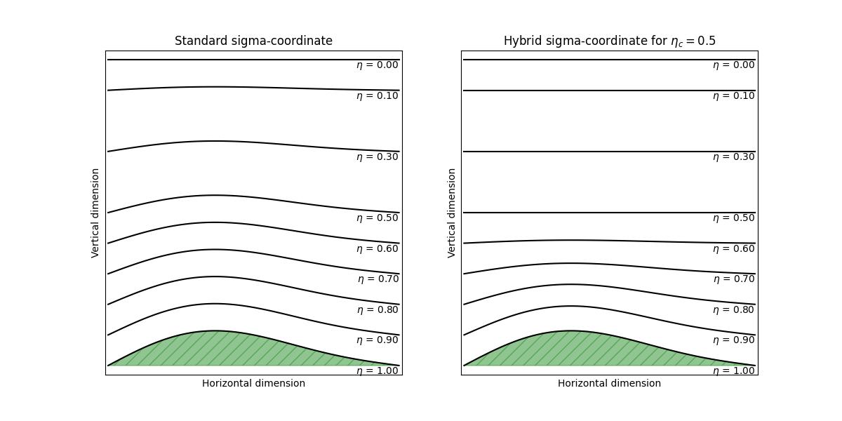
Standard sigma coordinates (left) vs. hybrid-sigma coordinates (right) for \(\eta_c = 0.5\). The horizontal and vertical dimensions are in arbitrary units of length. The green hatched section represents the surface of the Earth.#
The default value \(\eta_c\) used in the WRF model that produces the HRRR forecasts is \(\eta_c=0.2\), as can be seen from the user’s guide. The vertical coordinate otherwise is separated into 51 levels, including the top and bottom of the computational domain, with the specific values of \(\eta\) listed in the FAQ. As mentioned above, StormCast uses only a selected number of these vertical levels, which are enumerated in the paper [#6].
Earth2Studio#
The StormCast model is distributed as a part of the Earth2Studio software package, created by NVIDIA. This package makes it convenient to run StormCast inferences, as it can automatically download the necessary meso-scale initial data \(M_0\), as well as the synoptic scale low-resolution forecasts \(S_t\) that are required for running the model. Below we will show how to do this in practice and get StormCast running on AMD Instinct GPU Accelerators.
License#
StormCast comes bundled with Earth2Studio, released under the Apache License 2.0. Please see the full text of the license.
Installation#
To use StormCast on AMD Instinct GPUs, the easiest way is to use one of ROCm Docker images.
The Docker image we will use is
rocm/pytorch:rocm7.0.2_ubuntu24.04_py3.12_pytorch_release_2.8.0. If you have
Docker installed on your system, you can download this image simply by invoking the following:
docker pull rocm/pytorch:rocm7.0.2_ubuntu24.04_py3.12_pytorch_release_2.8.0
While it is not mandatory, you might also want to download the StormCast inference runner and plotter scripts we have provided: run-stormcast.py and plot-stormcast.py
Using the AMD Container Toolkit is recommended for running the image. If you have it installed, you can spin up a container running the image with the following command:
docker run -d \
    --runtime=amd \
    -e AMD_VISIBLE_DEVICES=all \
    --name stormcast \
    -v $(pwd):/workspace/ \
    rocm/pytorch:rocm7.0.2_ubuntu24.04_py3.12_pytorch_release_2.8.0 \
    tail -f /dev/null
Here we assume that you’ve downloaded the scripts above to your current working
directory, which will get mapped into the directory /workspace inside the
container.
If you do not have the AMD Container Toolkit installed, you can run the following command instead:
docker run -d \
    --device=/dev/kfd \
    --device=/dev/dri \
    --group-add video \
    --name stormcast \
    -v $(pwd):/workspace/ \
    rocm/pytorch:rocm7.0.2_ubuntu24.04_py3.12_pytorch_release_2.8.0 \
    tail -f /dev/null
When the container is running, you can now open a new interactive shell in the container by running the following:
docker exec -it stormcast /bin/bash
In the new session, move to the workspace directory and install the required Python dependencies by running the following:
cd /workspace
pip install earth2studio[stormcast] cartopy
You are now ready to run StormCast on your AMD Instinct hardware! Let’s see how to do that next.
Running inference#
To run StormCast inference with Earth2Studio you will need to import the necessary Python packages. The bare minimum required can be imported with:
import earth2studio.run as run
from earth2studio.models.px import StormCast
from earth2studio.data import HRRR
from earth2studio.io import ZarrBackend
To create a StormCast model with the default parameter values and settings you can then do the following:
package = StormCast.load_default_package()
model = StormCast.load_model(package)
This loads the default model from NVIDIA’s NGC registry. You will also need a data source for the model initial conditions. For StormCast, this is the HRRR analysis (not forecast) data source. Create this data source with:
data = HRRR()
Lastly, you will need a data backend for saving the model outputs. You can have Earth2Studio automatically save the model outputs into a Zarr dataset stored on the local disk by using the Zarr backend via:
io = ZarrBackend('model-output.zarr')
You can change the output file name to your liking.
Note
The Zarr outputs
are stored as directory hierarchies on your local drive, so this will create a
directory model-output.zarr/ under the directory /workspace/ in your
container, and thus also in the working directory from which you started the
container. Note also that the Zarr backend of Earth2Studio does not support
overwriting the outputs, so you will need to either change your output file name
or remove your existing output before trying to run inference again.
Now you can run StormCast inference starting from a date and time of your choosing for a number of one-hour time steps by running the following:
from datetime import datetime
starting_datetime = datetime(year=2025, month=1, day=1, hour=6)
nsteps = 6
io = run.deterministic([starting_datetime], nsteps, model, data, io)
This will run the deterministic part of StormCast for 6 one-hour time steps,
starting from 2025-01-01 06:00AM UTC. The resulting mean values will
automatically be saved into a Zarr output specified by io.
You will find that the StormCast model is fairly lightweight to run. On a single AMD MI300X GPU we found the deterministic model to take up approximately 5% of the available VRAM, or approximately 9.6 gigabytes. The runtime for six steps was less than two minutes.
Instead of scripting all of this yourself, you can use the run-stormcast.py
script we have provided. Using the script you can just
do the following:
python run-stormcast.py 2025-01-01T06:00 6
This will also run the deterministic part of StormCast for 6 one-hour time steps
starting from the same date and time as the Python code above, and will save the
output into outputs/pred-2025-01-01.zarr. Note that the output will be
automatically named based on the starting date of the inference, and
pre-existing outputs will be automatically overwritten.
Note
We will discuss the details of the generative part of StormCast in a future blog post. There we will also discuss some of the details and benefits of generative processing in weather prediction.
Plotting#
Once you have run StormCast and have the model outputs, it is easy to examine
and plot them using xarray and matplotlib. For this, we will need the
following additional Python imports:
import cartopy
import cartopy.feature
import cartopy.crs as ccrs
import matplotlib.pyplot as plt
import xarray as xr
First, we will need to specify the computational domain of the model. The StormCast model uses the HRRR grid, and the computational domain within it can be defined with the following:
hrrr_lat_lim: tuple[int, int] = (273, 785)
hrrr_lon_lim: tuple[int, int] = (579, 1219)
hrrr_lat, hrrr_lon = HRRR.grid()
model_lat = hrrr_lat[hrrr_lat_lim[0] : hrrr_lat_lim[1], hrrr_lon_lim[0] : hrrr_lon_lim[1]]
model_lon = hrrr_lon[hrrr_lat_lim[0] : hrrr_lat_lim[1], hrrr_lon_lim[0] : hrrr_lon_lim[1]]
This will yield the StormCast model grid using latitude and longitude. Note
that internally HRRR uses the
Lambert Conformal Conic projection
to define the data grid, but the function HRRR.grid() converts this to a
meshgrid defined with the usual WGS84 latitude and longitude coordinates.
However, for plotting purposes, we will still need the actual projection. This can be generated with the following:
projection = ccrs.LambertConformal(
    central_longitude=262.5,
    central_latitude=38.5,
    standard_parallels=(38.5, 38.5),
    globe=ccrs.Globe(semimajor_axis=6371229, semiminor_axis=6371229),
)
Now we can read in the StormCast outputs using the following:
ds = xr.open_zarr('model-output.zarr', consolidated=False)
Here we explicitly set consolidated=False since the Earth2Studio Zarr backend
does not do data consolidation. You can leave this out, but this may generate
warnings.
Next, generate the plot axis using:
fig, axis = plt.subplots(
    nrows=1,
    ncols=1,
    subplot_kw={'projection': projection},
    figsize=(5, 6),
    layout='compressed',
)
Note that you must supply the projection we defined before as an argument to plt.subplots().
Now we are ready to plot any of the variables forecasted by StormCast corresponding to any of the lead times we have forecasted for. For example, we can do the following:
variable = 'refc'
nstep = 2

data = ds[variable][0,nstep]

axis.pcolormesh(
    model_lon,
    model_lat,
    data,
    transform=ccrs.PlateCarree(),
    cmap='Spectral_r',
)

axis.coastlines()
axis.gridlines()
axis.add_feature(
    cartopy.feature.STATES.with_scale('50m'),
    linewidth=0.5,
    edgecolor='black',
    zorder=2,
)

plt.savefig('stormcast-plot.jpg')
This will plot the composite radar reflectivity as a heatmap, and also add
latitude-longitude gridlines, US coastlines and state borders on the plot.
Note that we have to use the PlateCarree projection here as this is the
compatible choice for the data produced by the HRRR.grid() method.
The final plot will be saved as the file stormcast-plot.jpg.
Running these commands should produce a figure like the one shown below.
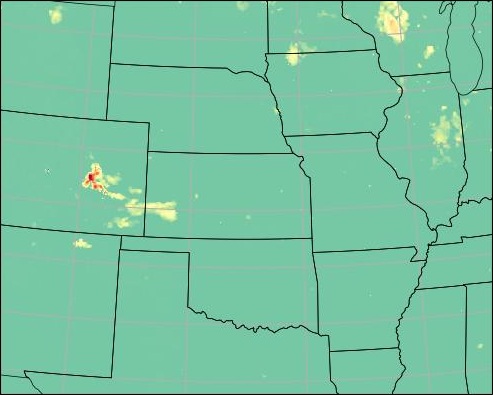
Example plot of StormCast output.#
However, this process can be automated using the plotter script
plot-stormcast.py that we’ve provided.
Using this script, you can plot the initial conditions and all the forecasted
lead times by simply invoking the
following:
python plot-stormcast.py outputs/pred-2025-01-01.zarr
This will produce a set of images with file names like
scast-2025-01-01-refc-frame-00.jpg and ...-frame-01.jpg and so on. The
images will contain the StormCast forecasts for the composite radar
reflectivity. They will also show the HRRR forecast as well as the HRRR analysis
ground truth data.
Note
Currently the plot-stormcast.py only plots the composite radar reflectivity,
but you can easily extend the code to plot any quantity you would like. Please
see the code and the comments therein.
Tip
If you have the ImageMagick open source image manipulation software installed, you can create a GIF animation of the individual frames by running:
convert -loop 0 -delay 150 scast-2025-01-01-*.jpg animation.gif
This will create a GIF file that will endlessly loop over the output frames, changing frame every 1.5 seconds. See below for an example.
Example animation showing the forecasted evolution of the composite radar reflectivity. Created from the outputs of the StormCast plotter program.#
Summary#
Numerical weather prediction is a computationally demanding enterprise, especially at the so-called meso-scales, where convective processes are important. Machine learning based weather prediction models offer an interesting new possibility to sidestep some of the problems faced by the traditional physics-based models. It is in this respect that NVIDIA’s StormCast, a convection-emulating machine learning based weather prediction model showcases some of the recent rapid progress in the field.
In this blog post we have briefly outlined the problem of weather prediction at different spatial and temporal scales. We discussed the problem of convection and thunderstorm prediction at meso-scales, and what difficulties this poses for traditional methods. We then presented StormCast, explained the basics of how the model works and how it partially solves some of these problems.
Finally, we showed how one can easily and efficiently run StormCast on AMD Instinct GPU Accelerators, and demonstrated how the predictions can be visualized. We also supplied a separate runner and plotter programs that the reader can use to quickly run and visualize larger sets of forecasts.
Look out for the next installments in our series of weather prediction blog posts. For example, we will further investigate and showcase the generative capabilities of StormCast when running on AMD hardware.
Acknowledgments#
During the writing, the author benefited from helpful comments from and discussions with Rahul Biswas, Luka Tsabadze and Sopiko Kurdadze.
Thumbnail image by user Memorialman, distributed at the Wikimedia Commons under the Creative Commons Attribution-Share Alike 4.0 International license.
We also acknowledge the freely available data produced by the HRRR and GFS teams, used for the StormCast inference runs.
Additional resources#
The StormCast runner program: run-stormcast.py
The StormCast plotter program: plot-stormcast.py
References#
[1] Orlanski, I. (1975). A Rational Subdivision of Scales for Atmospheric Processes. Bulletin of the American Meteorological Society, 56(5), 527–530. https://www.jstor.org/stable/26216020
[2] Roberts, C. D., Senan, R., Molteni, F., Boussetta, S., Mayer, M., and Keeley, S. P. E. (2018). Climate model configurations of the ECMWF Integrated Forecasting System (ECMWF-IFS cycle 43r1) for HighResMIP. Geosci. Model Dev., 11, 3681–3712. https://doi.org/10.5194/gmd-11-3681-2018
[3] Bryan, G. H., Wyngaard, J. C., & Fritsch, J. M. (2003). Resolution Requirements for the Simulation of Deep Moist Convection. Monthly Weather Review, 131(10), 2394-2416. https://doi.org/10.1175/1520-0493(2003)131<2394:RRFTSO>2.0.CO;2
[4] Dowell, D. C., Alexander, C. R., James, E. P., Weygandt, S. S., Benjamin, S. G., Manikin, G. S., Blake, B. T., Brown, J. M., Olson, J. B., Hu, M., Smirnova, T. G., Ladwig, T., Kenyon, J. S., Ahmadov, R., Turner, D. D., Duda, J. D., & Alcott, T. I. (2022). The High-Resolution Rapid Refresh (HRRR): An Hourly Updating Convection-Allowing Forecast Model. Part I: Motivation and System Description. Weather and Forecasting, 37(8), 1371-1395. https://doi.org/10.1175/WAF-D-21-0151.1
[5] Skamarock, W. C., Klemp, J. B. (2008). A time-split nonhydrostatic atmospheric model for weather research and forecasting applications. Journal of Computational Physics, 227, 7, 3465-3485. https://doi.org/10.1016/j.jcp.2007.01.037
[6] Pathak, J., Cohen, Y., Garg, P., Harrington, P., Brenowitz, N., Durran, D., Mardani, M., Vahdat, A., Xu, S., Kashinath, K., Pritchard, M. (2024). Kilometer-Scale Convection Allowing Model Emulation using Generative Diffusion Modeling. arXiv:2408.10958. https://doi:10.48550/arXiv.2408.10958
[7] Skamarock, W., Klemp, J., Dudhia, J., Gill, D. O., Liu, Z., Berner, J., Wang, W., Powers, J. G., Duda, M. G., Barker, D., & Huang, X.-Y. (2019). A Description of the Advanced Research WRF Model Version 4.1. https://doi.org/10.5065/1dfh-6p97
Disclaimers#
Third-party content is licensed to you directly by the third party that owns the content and is not licensed to you by AMD. ALL LINKED THIRD-PARTY CONTENT IS PROVIDED “AS IS” WITHOUT A WARRANTY OF ANY KIND. USE OF SUCH THIRD-PARTY CONTENT IS DONE AT YOUR SOLE DISCRETION AND UNDER NO CIRCUMSTANCES WILL AMD BE LIABLE TO YOU FOR ANY THIRD-PARTY CONTENT. YOU ASSUME ALL RISK AND ARE SOLELY RESPONSIBLE FOR ANY DAMAGES THAT MAY ARISE FROM YOUR USE OF THIRD-PARTY CONTENT.