Adaptive Top-K Selection: Eliminating Performance Cliffs Across All K Values on AMD GPUs#

Top-K selection is critical for LLMs and RAG workloads, yet standard Radix Sort implementations often suffer from performance cliffs at small K values due to fixed initialization overheads. In our AITER library (introduced in our previous blog [1]), we originally utilized an 11-bit radix sort for Top-K selection. While this approach excels at scale, we identified a critical efficiency gap for the lightweight filtering often required during modern inference.
In this blog, you will learn how to eliminate these bottlenecks on AMD MI300X GPUs. Specifically, we will explore how to:
Slash latency for small K by switching to register-based Bitonic Sort.
Unlock hardware potential using AMD’s DPP instructions and vectorized Buffer Loads.
Hide memory latency through efficient Double Buffering.
Implement an adaptive strategy that automatically selects the optimal algorithm for universal performance.
The Challenge with Radix Sort#
To understand the performance characteristics of radix sort across different K values, we profiled the Top-K kernels using performance counters on a workload with a sequence length of 3072 and FP32 elements. Figure 1 displays a plot of counter collection over time, comparing execution behavior for K=2048 and K=64.
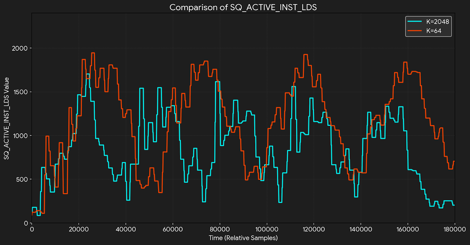
Figure 1. Performance Counter Comparison (K=2048 vs K=64)#
When profiling radix sort performance across different K values, we observed a counterintuitive phenomenon: the SQ_ACTIVE_INST_LDS[2] metric shows limited correlation with K. Even as K decreases substantially (e.g., from K=2048 to K=64), LDS activity remains consistently high. This occurs because radix sort’s histogram construction has a fixed cost—scanning all 2048 buckets and processing all input elements with atomicAdd operations on LDS—regardless of K. When K is small, most of these operations process non-top-K values, making them redundant from the perspective of the final result. To avoid this fixed overhead in small-K scenarios, we adopt bitonic-based algorithms that eliminate histogram construction and its associated LDS atomics entirely, scaling work proportionally with K.
Block-Level Top-K with Bitonic Sort#
Instead of strictly sorting the entire input, we implemented a family of warp-level algorithms that leverage bitonic sort, capitalizing on its favorable properties for GPU architectures.
Why Bitonic Sort?#
For small \(K\) values, bitonic sort presents a compelling alternative to radix sort. While radix sort typically achieves \(O(n \times d)\) complexity (where \(d\) represents the number of passes, typically 3 for 32-bit floats), its practical performance on GPUs is often bottlenecked by hardware constraints.
The critical insight lies in the hardware overhead. Radix-based selection relies heavily on histogram construction, which necessitates atomic operations on Local Data Share (LDS). Regardless of the candidate set size, this introduces a fixed overhead that becomes disproportionately expensive when \(K\) is small.
In contrast, our bitonic-based approaches—despite a theoretical complexity of \(O(n + K \log^2 K)\)—can operate primarily within registers using efficient intra-warp communication (DPP instructions)[3]. By eliminating slow memory accesses and atomic contentions on LDS, the register-based execution delivers superior performance. For small \(K\) values (e.g., \(K \le 128\)), the \(K \log^2 K\) term is negligible (amounting to just a few hundred operations), making the instruction-level parallelism of bitonic sort the clear winner.
Adaptive Strategy: BlockTopkSort vs BlockTopkFilter#
To maximize performance across different workload characteristics, we developed two complementary strategies:
BlockTopkSort: Optimized for scenarios where the input size per warp is relatively small. This strategy directly applies bitonic sort on register-resident data, leveraging DPP instructions for ultra-low-latency data exchange within warps, as illustrated in Figure 2.
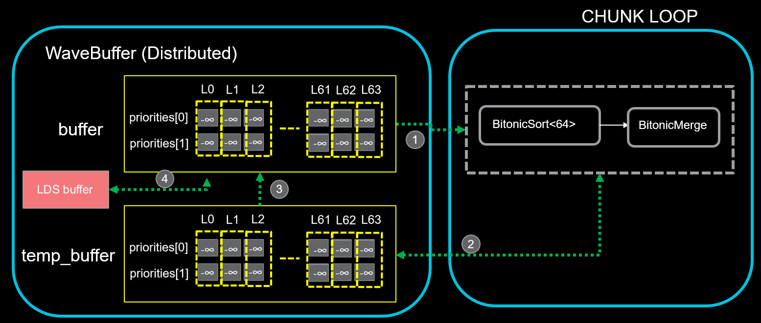
Figure 2. BlockTopkSort - Warp-Level Register Operations.#
Global Load & Sort: Load data from global memory into each lane’s buffer with a strided pattern (slots spaced by the warp size), then sort the priorities using a bitonic sort.
Warp Preparation: Strided warp load of priorities then in-place bitonic sort for merge readiness.
Register Merge: Element-wise compare the newly sorted chunk against the existing sorted buffer, overwriting entries where the new values are preferred.
Block-Wide Reduction: Tree reduction of top-k across wavefronts: upper half writes to LDS, lower half reads/merges; halve wavefronts each iteration until block-wide top-k.
BlockTopkFilter: Designed for larger input sizes where exhaustive sorting becomes expensive. This strategy employs a ballot-based filtering pass to aggressively prune candidates before sorting, reducing the effective problem size. Figure 3 shows this pipeline where only qualified elements proceed to the sorting stage.
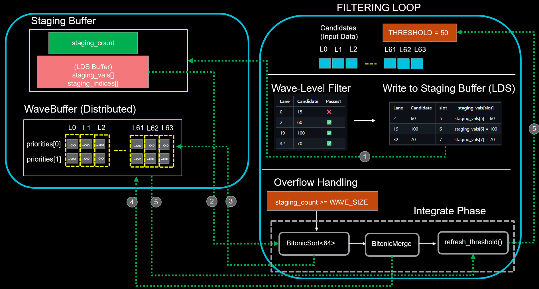
Figure 3. BlockTopkFilter Pipeline with Ballot-Based Candidate Pruning.#
Candidate Compaction: Use a parallel prefix sum (scan) to compact passing candidates into a staging buffer; trigger batch integration when the buffer holds 64 elements.
Sort: Perform a bitonic sort on 64 staged elements distributed across threads.
Prune: For each thread, compare the sorted value with its lowest-priority register element (priorities[slots_per_lane - 1]) and replace it if the new value is better.
Bitonic Merge: Use BitonicMerge to sort a bitonic sequence distributed across per-thread registers into a fully sorted sequence via logarithmic stages of compare–exchange operations.
Threshold Update: Update the filtering threshold by broadcasting the value of the k-th element to all lanes in the warp.
Hardware Acceleration with Opus Library#
To fully exploit AMD GPUs’ specialized hardware features, we leverage the Opus library[4]—a lightweight, single-header C++ DSL designed to bridge the gap between handwritten HIP kernels and highly-optimized template libraries like Composable Kernel. Opus provides essential abstractions that simplify low-level GPU programming while maintaining fine-grained control over performance-critical operations.
Why Opus?#
Opus offers precisely what we need for our Top-K implementation:
AMDGPU-specific data types with automatic conversion handling
Automated vectorized memory operations without manual implementation
Direct access to specialized GPU instructions (DPP, shuffle, med3) [3]
Minimal abstraction overhead while preserving code clarity
DPP (Data Parallel Primitives): For small-stride data exchanges (≤8 lanes apart), DPP instructions provide ultra-low-latency permutations within a warp:
T neighbor = opus::mov_dpp(value, opus::number<0xb1>(), ...); // Low-latency register exchange (significantly faster than shuffle)```
med3 Instruction: AMD’s median-of-3 hardware unit enables branch-free comparisons. By cleverly using a guard value, we turn compare-and-swap into a single instruction:
T selected = opus::med3(val_a, val_b, guard); // Replaces: (condition) ? val_a : val_b// Benefit: No branch divergence
These optimizations deliver up to 32% performance improvement over baseline implementations using standard shuffle and conditional instructions. For example, on the benchmark case of (Batch, Length, K) = (1024, 3072, 128) with float32 elements, the gains are particularly significant due to the high instruction efficiency requirements for small input sequences.
Addressing Memory Bottlenecks in Long-Context Scenarios#
As input sequences grow longer, memory access patterns become the dominant performance factor. Profiling our kernels on long-sequence workloads (e.g., Length = 131,072) revealed a critical bottleneck: the profiler’s hotspot analysis [5] showed significant time spent in IMMED category, predominantly consisting of s_waitcnt barriers waiting for global memory loads to complete. As shown in Figure 4, the profiler identifies IMMED instructions as the primary bottleneck for these long sequences.
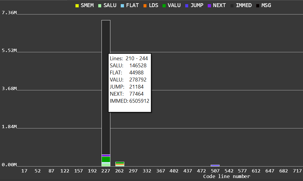
Figure 4. Hotspot Profile for Length=131,072#
To address this memory bottleneck, we implemented two optimizations:
Buffer Instructions – Vectorized memory access and buffer addressing to maximize bandwidth
Double Buffering – Software pipelining to hide memory latency
These techniques, detailed below, dramatically improve performance on long sequences.
Optimized Memory Access with Buffer Instructions#
We use AMD GPUs’ buffer_load_dwordx4 instruction for efficient memory access:
aiter::BufferResource buffer(data, size);
auto chunk = aiter::buffer_load_dwordx4(
    buffer.descriptor,  // 128-bit resource: base addr + range + config
    byte_offset,        // pointer offset
    cache_policy        // Explicit L1/L2 control
);
// Loads 16 bytes (4× float or 8× bf16) in single instruction**Buffer addressing mode** (per AMD RDNA3 ISA Section 9.4):
Uses a 128-bit buffer descriptor containing base address, range, and stride information
Supports offset-based indexing where the hardware computes the final address using the descriptor and provided offsets
Enables vectorized loads: fetches 4 dwords (16 bytes) per instruction
Key Benefits:
4-8× fewer load instructions: One buffer_load replaces multiple scalar loads
Bounds checking: Range field in descriptor enables hardware validation
Cache control: Explicit streaming hints for optimal cache behavior
The impact of buffer instructions is particularly significant for large input sequences. On the configuration (Batch, Length, K) = (1024, 131072, 128) with float32 elements, the optimization delivers up to 55% performance improvement over scalar pointer-based loads, demonstrating the critical importance of memory access efficiency for long-context workloads.
Memory Latency Hiding with Double Buffering#
Global memory access latency can severely bottleneck performance. We employ a double buffering strategy to overlap memory loads with computation:
Dual Buffers: Maintain two register arrays – one for active processing, one for prefetching
Software Pipelining: While processing chunk N, asynchronously load chunk N+1
Zero Stalls: By the time chunk N finishes, chunk N+1 is ready in registers
Implementation Comparison#
To illustrate the impact, let’s compare a standard implementation versus our double-buffered approach.
1. Baseline: No Prefetch (Serial Execution)#
In the naive implementation, the kernel issues a load request and immediately attempts to use that data. This forces the GPU to insert s_waitcnt barriers to stall execution until the memory transaction completes, fully exposing global memory latency.
// Baseline: Serial Load-Process
VecType reg;
for (...) {
    // 1. Issue Load: VMEM instruction
    reg = buffer_load(current_offset);

    // 2. STALL: Must wait for 'reg' to be ready

    // 3. Compute: VALU instruction
    process(reg);

    current_offset += stride;
}
2. Optimization: Double Buffering (Prefetch)#
In the optimized version, we preload the first chunk before the loop starts. Inside the loop, we issue the load for the next iteration (arr[1]) before we start processing the current data (arr[0]).
// Optimization: Double Buffering
VecType arr[2];

// Prologue: Pre-load chunk 0
arr[0] = buffer_load(offset);

for (...) {
    // 1. Prefetch: Asynchronously load chunk N+1 into the back buffer
    arr[1] = buffer_load(next_offset);

    // 2. Compute: Process chunk N (in front buffer) immediately
    // The latency of loading arr[1] is hidden behind this computation
    process(arr[0]);

    // 3. Swap: Rotate buffers for the next iteration
    arr[0] = arr[1];
}
We can verify the efficacy of this optimization by examining the Instruction Timing trace (as shown in the figure below).
Without Prefetch (Top Timeline): The unoptimized trace reveals the cost of latency. After every Yellow VMEM block (load issue), there is a significant empty gap (pipeline stall) before the Green VALU block begins. The compute units are forced to wait for the data to travel from memory to registers, resulting in poor utilization and longer overall execution time.
With Prefetch (Bottom Timeline): Looking at the optimized trace, we see a highly efficient pipeline. The Yellow blocks (VMEM instructions) represent the memory loads running in the background. Crucially, notice how the Green blocks (VALU instructions)—the actual computation—are tightly packed in the middle. The Compute Unit is able to execute these Green compute instructions while the VMEM instructions are in flight. The memory latency is effectively “hidden” behind the compute work, keeping the execution units saturated.
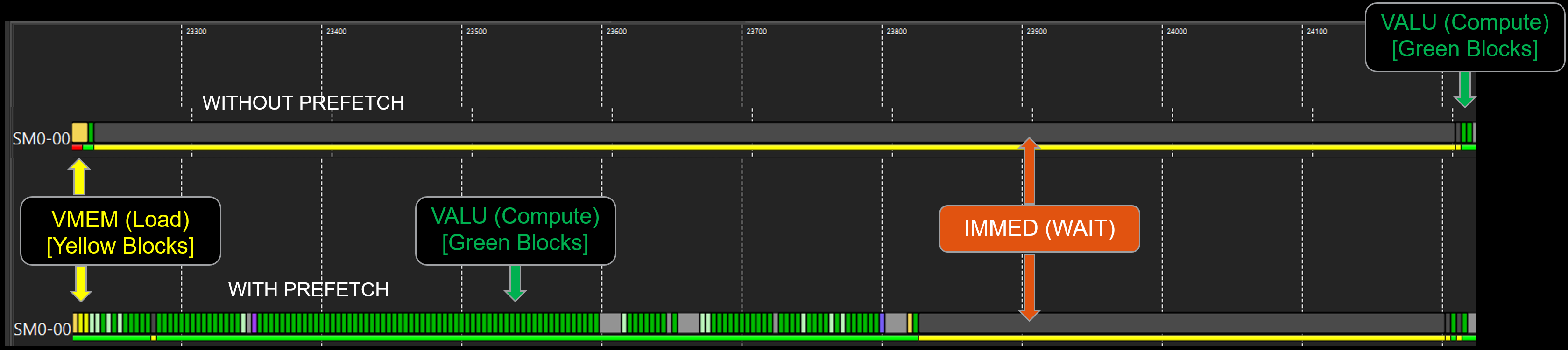
Figure 5. Instruction Timing Trace Comparison – Without Prefetch (Top) vs. With Prefetch (Bottom)#
Adaptive Strategy Selection#
While both radix sort-based Top-K and bitonic-based BlockTopK exhibit O(n) asymptotic complexity (where n is the sequence length), their practical performance characteristics differ significantly.
Complexity Comparison#
Radix Sort-Based Top-K:
Requires 3 passes over the input to process 32-bit floats (11-bit radix per pass)
Fixed histogram overhead remains constant regardless of K
Effective complexity: O(3n)
Bitonic-Based BlockTopK:
Single-pass input scan followed by bitonic sort/merge
Performance scales with the selected K value
Effective complexity: O(n + K log² K)
The fundamental trade-off: radix sort’s cost is K-independent, while bitonic sort becomes more expensive as K grows.
Determining the Optimal Threshold#
To find the perfect switching point, we need to balance the math. We looked for the crossover point where the cost of bitonic sort exceeds the fixed overhead of radix sort:
This suggests that for small K relative to n, bitonic sort should be preferred.
Empirical Refinement#
We validated this formula on AMD MI300X across sequence lengths ranging from 3,072 to 131,072. While the basic inequality holds well for n ≤ 16,384, it does not fully account for the additional performance impact of longer sequences on Block-Level Top-K.
We observed that as input sequences grow beyond this threshold, the accumulated overhead of scanning n elements impacts Block-Level Top-K more significantly than initially estimated. To capture this behavior, we introduce a length-dependent adjustment tuned specifically for MI300X:
where:
This empirically-derived factor captures the observed scaling behavior:
At n = 8,192: Factor ≈ 0.79 → threshold K ≈ 195
At n = 65,536: Factor ≈ 0.579 → threshold K ≈ 576
At n = 131,072: Factor ≈ 0.546 → threshold K ≈ 878
Figure 6 illustrates the adaptive threshold K as a function of sequence length n, derived from our MI300X-tuned Factor(n) formula. Each point on the curve represents the minimum K value at which radix sort-based Top-K becomes more efficient than Block-Level Top-K for a given sequence length. For K values above this threshold, we switch to radix sort-based algorithms to achieve optimal performance. The curve demonstrates that as sequences grow longer, the crossover point shifts to higher K values, reflecting the changing performance dynamics between the two algorithmic approaches.
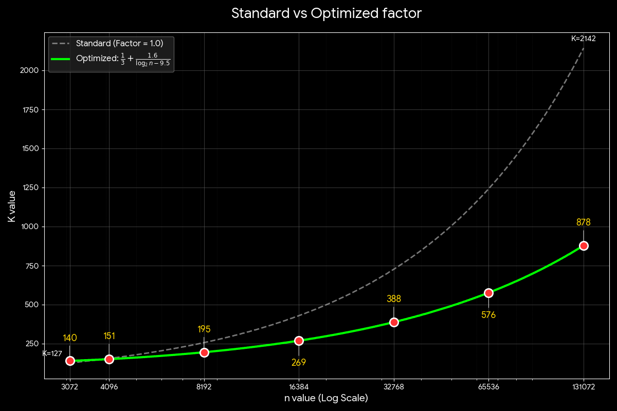
Figure 6. Adaptive K Threshold Curve#
Performance Evaluation#
To validate our adaptive strategy, we conducted comprehensive benchmarking on AMD MI300X GPUs using ROCm™ 7.0. We compared our implementation against the following baselines:
PyTorch native (
torch.topk, v2.8.0): Reference implementation leveraging rocPRIM for GPU primitivesTriton (v3.4.0): AITER’s Triton-based Top-K implementation with adaptive algorithm selection
radix_11bits: HIP-based 11-bit radix sort baseline
All experiments use FP32 elements with varying sequence lengths (3,072 to 131,072) and K values (1 to 2,048).
Figure 7 illustrates the performance comparison across different Top-K strategies. The dashed line represents BlockTopK (our bitonic sort-based implementation), which demonstrates competitive performance for K ≤ 128 but begins to lag behind the radix sort-based approach (radix_11bits) as K increases beyond this threshold.
Our AdaptiveTopK strategy intelligently selects the optimal algorithm based on K: leveraging BlockTopK for K ≤ 128 and switching to radix_11bits for K > 128. This adaptive selection ensures peak performance across the entire K spectrum, as evidenced by the solid line consistently matching or exceeding the best-performing algorithm at each K value.
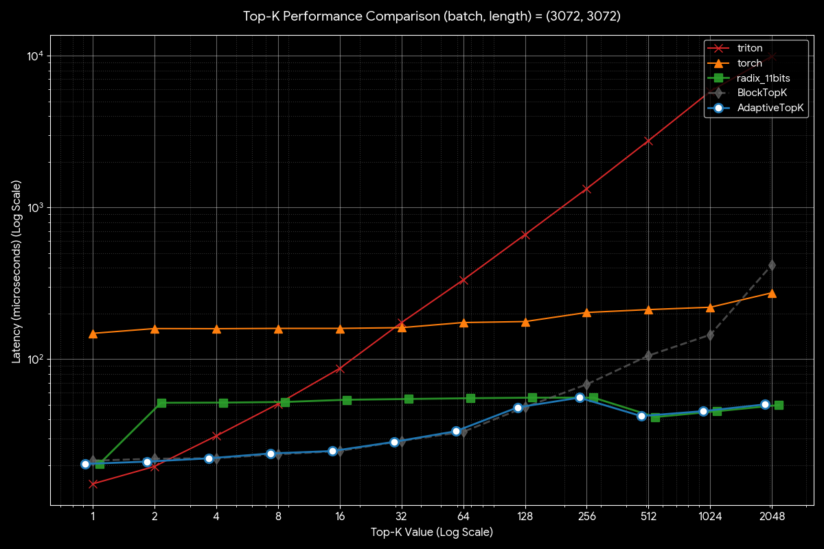
Figure 7. Performance Across Different K Values#
Building on this validation, Figure 8 directly compares AdaptiveTopK against other state-of-the-art implementations across varying sequence lengths for K = 64. AdaptiveTopK consistently delivers superior performance across all tested sequence lengths, demonstrating the effectiveness of our bitonic sort-based strategy for small K values.
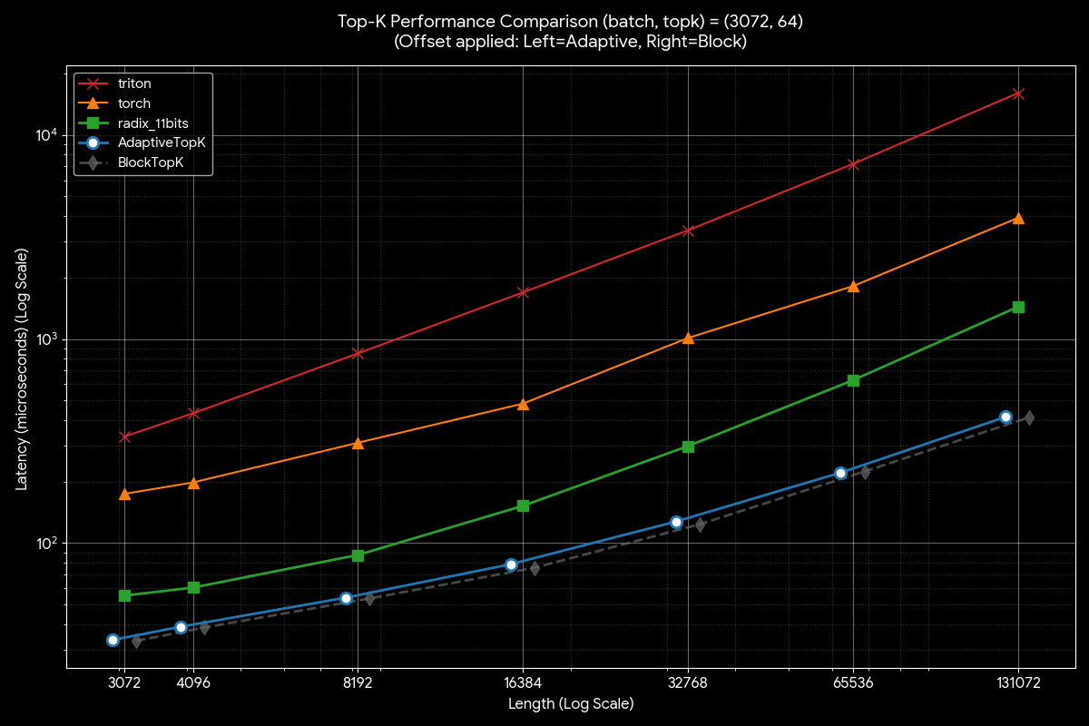
Figure 8. AdaptiveTopK Performance for Small K (K = 64)#
Figure 9 presents the comparison for K = 2048, where AdaptiveTopK seamlessly matches the performance of radix_11bits. This confirms that our adaptive threshold correctly identifies when to switch algorithms, ensuring optimal performance for large K values as well.
These results validate our adaptive strategy: by dynamically selecting between bitonic sort and radix sort based on K, we achieve optimal performance across diverse workload configurations without requiring manual algorithm selection.
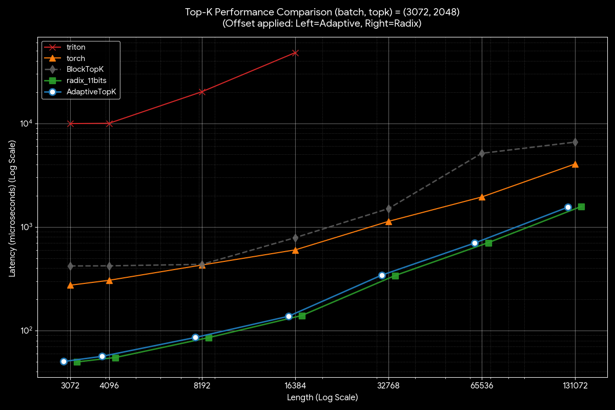
Figure 9. Performance Comparison for Large K (K = 2048)#
Summary#
This blog post presents an adaptive Top-K selection strategy optimized for AMD GPUs. We demonstrate how bitonic-based algorithms (BlockTopkSort and BlockTopkFilter) leverage AMD GPU-specific optimizations—including DPP instructions for ultra-low-latency data exchange, med3 for branch-free comparisons, buffer instructions for vectorized memory access, and double buffering for latency hiding—to deliver excellent performance for small K values.
However, as K grows larger, the bitonic sort’s O(K log² K) term becomes dominant. To address this, we switch to radix-based algorithms, which maintain consistent performance regardless of K due to their fixed histogram processing cost.
The key challenge lies in determining the optimal switching threshold. We present an empirically-derived formula tuned for AMD MI300X that accounts for both K and sequence length n, enabling intelligent algorithm selection across diverse workload configurations.
The resulting AdaptiveTopK implementation dynamically selects the best-performing algorithm based on runtime parameters, ensuring optimal performance across the entire spectrum of Top-K scenarios—from small K where bitonic sort excels, to large K where radix sort dominates—without requiring users to manually select algorithms.
We invite you to try out the AdaptiveTopK implementation in your own workloads. Check out the code in the latest AITER GitHub repository linked below [6], and let us know how it performs on your models!
References#
[1] AITER Library
[2] MI300 and MI200 Series performance counters and metrics
[3] AMD Instinct MI300 Instruction Set Architecture Reference Guide
[6] AdaptiveTopK
Disclaimers#
Third-party content is licensed to you directly by the third party that owns the content and is not licensed to you by AMD. ALL LINKED THIRD-PARTY CONTENT IS PROVIDED “AS IS” WITHOUT A WARRANTY OF ANY KIND. USE OF SUCH THIRD-PARTY CONTENT IS DONE AT YOUR SOLE DISCRETION AND UNDER NO CIRCUMSTANCES WILL AMD BE LIABLE TO YOU FOR ANY THIRD-PARTY CONTENT. YOU ASSUME ALL RISK AND ARE SOLELY RESPONSIBLE FOR ANY DAMAGES THAT MAY ARISE FROM YOUR USE OF THIRD-PARTY CONTENT.