From Theory to Kernel: Implement FlashAttention-v2 with CK-Tile#

In our previous blog, Hands on with CK Tile we walked through how to build a basic GEMM kernel using CK-Tile. In this blog, we will further explore the implementation of a fused kernel, specifically introducing the FlashAttention (FA)-v2 forward kernel. Figure 1 provides an overview of the FlashAttention kernel executions and data movements that occur during the computation of a single thread block of output matrix. Each of the subsequent sections explains details on how to implement this using CK-Tile.

Figure 1. FlashAttention kernel execution overview#
What is a Fused kernel?#
In GPU programming, each kernel launch introduces overhead. Performing multiple operations in sequence with separate kernel launches increases latency, and storing intermediate results in global memory further slows down execution due to the relatively high cost of global memory access. A Fused Kernel basically combines multi small kernels into the fused one, so that to minimize multiple small kernels launch time and reduce data movement latency among these small kernels. FlashAttention is a fused kernel, but it’s not a trivial composition—it’s a highly optimized, memory-efficient implementation of the attention mechanism used in transformer models. Let’s now focus on how to implement FlashAttention.
Problem Define#
The goal is to compute the attention mechanism, a core operation in transformer architectures. To keep the implementation of the FlashAttention kernel simple and focused, we selected the following problem shape.
Batch  = 64;   # Batch Number * Head Number
M0     = 4096; # Sequence Length for Q
N0     = 4096; # Sequence length for KV
K0     = 128;  # Q/K Head Dimension
N1     = 128;  # V/O Head Dimension
The overall computation with tensor shape is as following:
S[M0, N0] = Q[M0, K0] * K[N0, K0].TP[M0, N0] = Softmax(S[M0, N0])O[M0, N1] = P[M0, N0] * V[N1, N0].T
Problem Division#
In this section we will help you to grasp how the FlashAttention kernel maps the problem with GPU hardware. To map the large attention computation problem onto GPU Compute Units (CUs) by dividing it into tiles. Each tile is processed by a workgroup. The matrices involved are large, so we partition them into smaller tiles (submatrices) that can be processed in parallel by different GPU workgroups. The following workgroup level tile size is used. Below numbers provide how much each tensor a workgroup will handle at a time.
kM0PerBlock = 128  # Tile size in M (rows of Q)
kN0PerBlock = 128  # Tile size in N (columns of K)
kK0PerBlock = 32   # Tile size in shared dimension (Q and K)
kN1PerBlock = 128  # Tile size in N1 (columns of V and output O)
kK1PerBlock = 32   # Tile size in shared dim for V
Problem Size |
sub-Block Size |
Intra-ThreadBlock Loop Over |
Inter-ThreadBlock Parallelism |
|---|---|---|---|
|
|
No |
Yes |
|
|
Yes |
No |
|
|
Yes |
No |
|
|
No |
Yes |
Consider how a single workgroup completes the computation of one block [kM0PerBlock, kK1PerBlock] of output O, it basically requires one block of Q, but the whole K, V tensor. As each time, only [kN0PerBlock, kK0PerBlock] of K and [kN1PerBlock, kK1PerBlock] of V can be loaded, so there needs intra-threadblock loop over K, V. And for each block in the final output O is mapping to an individual workgroup, which gives inter-threadblock parallelism over Q as shown in Figure 2.
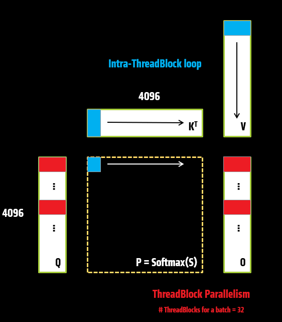
Figure 2. Workgroup level tiling#
Data Movement and Memory Abstraction#
From a memory perspective, all input tensors (Q, K, V) are initially stored in DRAM (global memory), and the output tensor (O) is ultimately written back to DRAM. Because the computation involves looping over the K and V tensors—operations that are highly bandwidth-sensitive—it is more efficient to prefetch K and V into LDS (local data share) to reduce global memory access latency.
The following tensors on DRAM and LDS are defined:
// Q, K, V, O DRAM
const auto q_dram = make_naive_tensor_view<global>(q_ptr, make_tuple(M0, K0), make_tuple(StrideQ, 1), number<32>{}, number<1>{});
const auto k_dram = make_naive_tensor_view<global>(k_ptr, make_tuple(N0, K0), make_tuple(StrideK, 1), number<32>{}, number<1>{});
const auto v_dram = make_naive_tensor_view<global>(v_ptr, make_tuple(N0, K0), make_tuple(StrideV, 1), number<32>{}, number<1>{});
auto o_dram = make_naive_tensor_view<global>(o_ptr, make_tuple(M0, N1), make_tuple(StrideO, 1), number<32>{}, number<1>{});

// K, V LDS
auto v_lds = make_tensor_view<lds>(reinterpret_cast<VDataType*>(smem_ptr),  MakeVLdsBlockDescriptor());
auto k_lds = make_tensor_view<lds>(static_cast<BDataType*>(smem_ptr), MakeBLdsBlockDescriptor());
The bottom execution of MFMA instructions require input tensors on on-chip memories (VGPRs or LDS), so next the step is to define data movement from DRAM to on-chip memories:
Q tensor written from DRAM to VGPRs, used as mfma inputs
K tensor written from DRAM to LDS, then load from LDS to VGPRs, used as mfma inputs
V tensor written from DRAM to LDS, used as mfma inputs
As the data movement is processed by lanes, the concept TileDistribution is used to describe the lane-data-mapping in workgroup-level in CK-Tile:
// q, k, v, o dram_window
auto q_dram_window = make_tile_window(q_dram, make_tuple(kM0PerBlock, kK0PerBlock), {iM0, 0}, MakeADramTileDistribution()) ;
auto k_dram_window = make_tile_window(k_dram, make_tuple(kN0PerBlock, kK0PerBlock), {0, 0}, MakeBDramTileDistribution()) ;
auto v_dram_window = make_tile_window(v_dram, make_tuple(kN1PerBlock, kK1PerBlock), {iN1, 0}, MakeVDramTileDistribution()) ;
auto o_dram_window = make_tile_window(o_dram, make_tuple(kM0PerBlock, kN1PerBlock), {iM0, iN1}, o.get_tile_distribution());
Data movement to and from LDS is similar to the previous case, but with one key difference: LDS typically operates on 128-bit cache lines for efficient access. As a result, additional alignment is required when mapping the logical tensor shape to LDS memory. Afterward, a merge transformation is applied to restore the original logical tensor layout from the optimized LDS memory format.The concept Lds_block_descriptor is used for this processing.
In general, lds_windows is separated as 2 individual windows: write_lds_window and load_lds_window, as write to and load from can use different tile distributions, which is the case for K Tensor. For V Tensor, v_lds_window is used directly as mfma input, as showed in following:
// k lds_window
constexpr auto b_lds_block_desc = Policy::template MakeBLdsBlockDescriptor<Problem>();
auto k_lds_block = make_tensor_view<lds>(k_lds, b_lds_block_desc);
auto k_copy_lds_window = make_tile_window(k_lds_block, make_tuple(kNPerBlock, kKPerBlock), {0, 0}, k_dram_window.get_tile_distribution());
auto k_lds_gemm_window = make_tile_window(k_lds_block, make_tuple(number<kNPerBlock>{}, number<kKPerBlock>{}), {0, 0});
// v lds_window
auto v_lds_window = make_tile_window(v_lds, make_tuple(kN1PerBlock, kK1PerBlock), {0, 0});
Let’s zoom in a bit more, the intermediate output tensor C from gemm0 and gemm1 need prepare its memory layout in workgroup level as well. The memory abstraction here is combined by outer(inter-warps) tile distribution and inner(intra-warp) tile distribution.
Take an example with workgroup level C tile as shown via Figure 3: C[kM0PerBlock, kN0PerBlock], the outer tile distribution defines warps layout along each dimension and the number of loops of each warp; while the inner tile distribution define lanes layout, repeats of lanes, and vector load size per lane inside warp, which is defined inside WarpGemm(WG) instance. Once combining outer and inner tile distribution, a unified descriptor c_block_dstr_encode is used for lanes-data-mapping at workgroup level.
constexpr auto c_block_outer_dstr_encoding = tile_distribution_encoding<
    sequence<>,
    tuple<sequence<MIterPerWarp, MWarp>, sequence<NIterPerWarp, NWarp>>,
    tuple<sequence<1, 2>>,
    tuple<sequence<1, 1>>,
    sequence<1, 2>,
    sequence<0, 0>>{};

auto c_block_dstr_encode = make_embed_tile_distribution_encoding(c_block_outer_dstr_encoding, WG::CWarpDstrEncoding{});
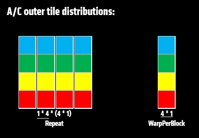
Figure 3. Tile Distribution Descriptor#
Finally, lets explain q_reg_tensor. As mentioned previously, to compute one block of output C, it requires loading one block tile of Q tensor, and loops over the whole K, V tensors. During this processing, actually once the 1st block of output C is done, the whole block-level tile Q, a.k.a q_reg_tensor is already in VGPRs. So in later loops, q_reg_tensor is ready for mfma inputs, no more Q data movement is needed.
constexpr auto a_reg_block_dstr = Policy::template MakeARegBlockDescriptor<Problem>();
auto a_copy_reg_tensor = make_static_distributed_tensor<ADataType>(a_reg_block_dstr);
ARegBlockDescriptor is packaged in the same way as c_block_dstr_encode by combining inter-warps and intra-warp tile distributions.
Computation Pipeline#
After all the memory layouts and data access patterns are carefully defined, the actual computation proceeds in two structured layers. Once all tensor memory layout and access patterns are well defined from the previous section, the computation can be considered as 2 levels
loops along blocks of output C a.k.a the inter-threadblock parallelism,
computes each block of output C by looping over K and V tensor,a.k.a the intra-threadblock loops.
The following pseudocode illustrates the overall computation pipeline:
M0, N1 = O.shape
N0, K0 = K.shape
num_c_blocks = M0 // kM0PerBlock
num_k_blocks = N0 // kN0PerBlock
num_v_blocks = N0 // kN1PerBlock
assert num_k_blocks==num_v_blocks
for c_block_idx in range(num_c_blocks):
    q_reg_tensor = load_q_dram(c_block_idx)
    for k_block_idx in range(num_k_blocks):
        k_lds_tensor = load_k_buffer(k_block_idx)
        s[c_block_idx, k_block_idx] = BlockGemm0(q_reg_tensor, k_lds_tensor)
        p[c_block_idx, k_block_idx] = SOFTMAX(s[c_block_idx, k_block_idx])
    for v_block_idx in range(num_v_blocks):
        v_lds_tensor = load_v_buffer(v_block_idx)
        acc[c_block_idx] += BlockGemm1(p[c_block_idx, v_block_idx], v_lds_tensor)
return acc
The CK-Tile implementation closely follows this logic. Each stage of the FlashAttention algorithm maps directly to a block of code in the kernel:
// loop over Column of S (J loop)
do
{
    // 1. on chip, compute S[i, j] = Q[i] * KT[j]
    s_acc = gemm0_pipeline(k_dram_window, q_reg_tensor, smem_ptr);

    // 2.1 on chip, compute m[i, j] = max(m_old[i], rowmax(s[i, j]))
    m_local = block_tile_reduce<SMPLComputeDataType>(s, sequence<1>{}, f_max, std::numeric_limits<SMPLComputeDataType>::lowest());
    block_tile_reduce_sync(m_local, f_max, WithBroadcast=True);
    m_old = m ;
    tile_elementwise_inout([](auto& e0, auto e1, auto e2){e0 = max(e1, e2); } m, m_old, m_local);

    // 2.2 on chip, compute p[i, j] = exp(s[i, j] - m[i, j])
    auto p_compute = make_static_distributed_tensor<SMPLComputeDataType>(s.get_tile_distribution());
    constexpr auto p_spans = decltype(p_compute)::get_distributed_spans();
    sweep_tile_span(p_spans[I0], [&](auto idx0){
        constexpr auto i_idx = make_tuple(idx0);
        sweep_tile_span(p_spans[I1], [&](auto idx1){
            constexpr auto i_j_idx = make_tuple(idx0, idx1);
            p_compute(i_j_idx) = exp(s[i_j_idx] - m[i_idx]);
        });
    })

    // 2.3 on chip, compute l[i, j] = exp(m_old[i] - m[i]) * l_old[i] + rowsum(p[i, j])
    auto rowsum_p = block_tile_reduce<SMPLComputeDataType>(p_compute, sequence<1>{}, f_sum, SMPLComputeDataType{0});
    block_tile_reduce_sync(rowsum_p, f_sum);
    sweep_tile_span(p_spans[I0], [&](auto idx0){
        constexpr auto i_idx = make_tuple(idx0);
        const auto tmp = exp(m_old[i_idx] - m[i_idx]);
        l[i_idx] = tmp * l[i_idx] + rowsum_p[i_idx] ; //per row
        // o_acc 1st half update
        sweep_tile_span(p_spans[I1], [&](auto idx1){
            constexpr auto i_j_idx = make_tuple(idx0, idx1);
            o_acc(i_j_idx) *= tmp ;
        })
    })

    // 3. on chip, compute o_acc[i, j] = exp(m_old[i] - m[i]) * o_acc[i, j] + p[i] * v[j]
    // o_acc 2nd half update
    static_for<0, k1_loops-1, 1>{}(([&] auto i_k1){
        v = load_tile(v_dram_window) ;
        block_sync_lds();
        gemm1(o_acc, get_slice_tile(p,  sequence<0, i_k1 * kK1PerBlock>{}, sequence<kM0PerBlock, (i_k1+1)*kK1PerBlock>{}), v_lds_window);
        block_sync_lds();
    })

    // 4. on chip, compute o_acc[i] = o_acc[i] / l[i]
    o_spans = decltype(o_acc)::get_distributed_spans();
    sweep_tile_span(o_spans[I0], [&](auto idx0){
        constexpr auto i_idx = make_tuple(idx0);
        tmp = 1 / l[i_idx];
        sweep_tile_span(o_spans[I1], [&](auto idx1){
            constexpr auto i_j_idx = make_tuple(idx0, idx1);
            o_acc[i_j_idx] *= tmp;
        });
    });

    // 5. write to HBM as the i-th block of o_acc
    store_tile(o_dram_window, o_acc);
}
Summary#
In this blog, you learned how to implement a high-performance FlashAttention-v2 kernel using CK-Tile, leveraging fused operations and efficient memory tiling. FlashAttn-v2 serves as an excellent example of how CK-Tile empowers efficient development of custom kernels. With approximately 100 lines of CK-Tile code, the complex FlashAttention algorithm can be implemented effectively and efficiently. For more advanced optimizations, particularly in attention kernels, the FMHA sample is also worth exploring. CK-Tile provides a structured way to map each stage of the FlashAttention pipeline to well-defined memory movement and compute steps.
ROCm vs. CUDA Terminology Reference#
Here is a mapping table from CUDA to ROCm
Concept |
CUDA(NVIDIA) |
ROCM(AMD) |
|---|---|---|
Thread |
Thread |
Work-item |
Warp |
Warp (32 threads) |
Wavefront (64 work-item) |
Thread Block |
Block |
Work Group |
Shared Memory |
Shared Memory |
LDS (Local Data Share) |
Global Memory |
Global Memory |
Global Memory |
Registers |
Register |
VGPR, SGPR |
Compute Units |
SM (Streaming Multiprocessor) |
CU (Compute Unit) |
Accelerators |
Tensor Core |
Matrix Core |
Parallel Strategy |
SIMT (single-instruction, multi-threads) |
SIMD (single-instruction, multi-data) |
Acknowledgement#
We extend our special thanks to the AMD CK Core team members for their valuable support and contributions.
Additional Resources#
Disclaimers#
Third-party content is licensed to you directly by the third party that owns the content and is not licensed to you by AMD. ALL LINKED THIRD-PARTY CONTENT IS PROVIDED “AS IS” WITHOUT A WARRANTY OF ANY KIND. USE OF SUCH THIRD-PARTY CONTENT IS DONE AT YOUR SOLE DISCRETION AND UNDER NO CIRCUMSTANCES WILL AMD BE LIABLE TO YOU FOR ANY THIRD-PARTY CONTENT. YOU ASSUME ALL RISK AND ARE SOLELY RESPONSIBLE FOR ANY DAMAGES THAT MAY ARISE FROM YOUR USE OF THIRD-PARTY CONTENT.