Elevating 3D Scene Rendering with GSplat

October 03, 2025 by Deeksha Goplani, Ish Kool, Karthik Kashyap Thatipamula, Marco Grond, Mark Granroth-Wilding, Pier Luigi Dovesi, Shaghayegh Roohi, Vish Vadlamani, Vikas C Sajjan, Phani Vaddadi.

5 min read. | 1111 total words.

Software tools & optimizations

Computer Vision, PyTorch

Developers

In this blog we explore how to use GSplat, a GPU-optimized Python library for training and rendering 3DGS models, on AMD devices. This tutorial will guide you through training a model of a scene from a set of captured images, which will then allow you to render novel views of the scene. We use a port of the original GSplat code that has been optimized for AMD GPUs. The examples used throughout this blog were trained and rendered using an AMD MI300X GPU.

We present step-by-step instructions to train a model with GSplat, as well as how to render novel views. We further present an in depth look into the inner workings of a 3DGS model during this process. Finally, we report performance statistics on standard benchmarks, highlighting the benefits of running GSplat on AMD MI300X GPUs.

3D Gaussian Splatting (3DGS) is a novel and highly efficient technique for real-time rendering of 3D scenes trained from a collection of multiview 2D images of the scene. It has emerged as an alternative to neural radiance fields (NeRFs), offering significant advantages in rendering speed while maintaining comparable or even superior visual quality. Unlike NeRFs which represent a scene as a continuous volumetric function implicitly embedded in the network’s parameters, 3DGS models a scene as a collection of 3D Gaussians, or splats which are parameterized by position, scale, orientation, color, and opacity. This simple yet powerful representation allows for direct and rapid rendering, making it ideal for interactive applications, such as virtual/augmented reality and autonomous driving.

Some key features of 3DGS, that make it an attractive option for a variety of applications, include:

• Real-time rendering: By representing the scene with a discrete set of 3D Gaussians and leveraging GPU rasterization, 3DGS enables highly parallel and efficient rendering, perfectly suited to modern GPU architectures.

• High fidelity and quality: Despite its simplicity, 3DGS achieves high-quality reconstructions of static scenes, accurately capturing fine textures and visual details. While it approximates geometry rather than modeling it explicitly, the results are visually compelling for many real-world applications.

• Explicit scene representation: Unlike NeRFs, 3DGS uses an explicit, discrete set of primitives to represent objects and surfaces. The scene representation is thus interpretable and easy to manipulate. Artists and developers can directly edit, add, or remove splats and trained scenes can be combined.

• Efficient training: As a consequence of the fast rendering process, training a 3DGS scene model from a set of images is remarkably fast and efficient, often taking minutes on a modern GPU, depending on scene complexity and image resolution.

A primer on Gaussian Splatting

3D Gaussian Splatting (3DGS) provides an explicit, point-based volumetric representation of a scene. It represents a scene using a sparse set of 3D multivariate anisotropic Gaussian primitives, each defined by mean position, a covariance matrix defining its shape and orientation, color (via spherical harmonics), and opacity. The color is modeled using spherical harmonics, a set of functions that represent directional variations on a sphere, with a base component representing the view-independent color and additional higher-order coefficients capturing the view-dependent appearance, i.e. how an object’s appearance changes when viewed from different angles. Opacity controls how much each Gaussian blocks or contributes light. When rendering a pixel, 3DGS accumulates color contributions from all Gaussians along the ray. Opacity acts as a weight for each Gaussian’s color in this accumulation. 3DGS enables real-time rendering of the scene by projecting 3D Gaussians onto the image plane, i.e. rasterizing them, and blending their contribution to produce the final view of the scene. 3DGS starts from an initial set of 3D points, which may be randomly sampled or derived from sources such as COLMAP or LiDAR. The 3DGS process of mapping and rendering an object is shown in the figure below.

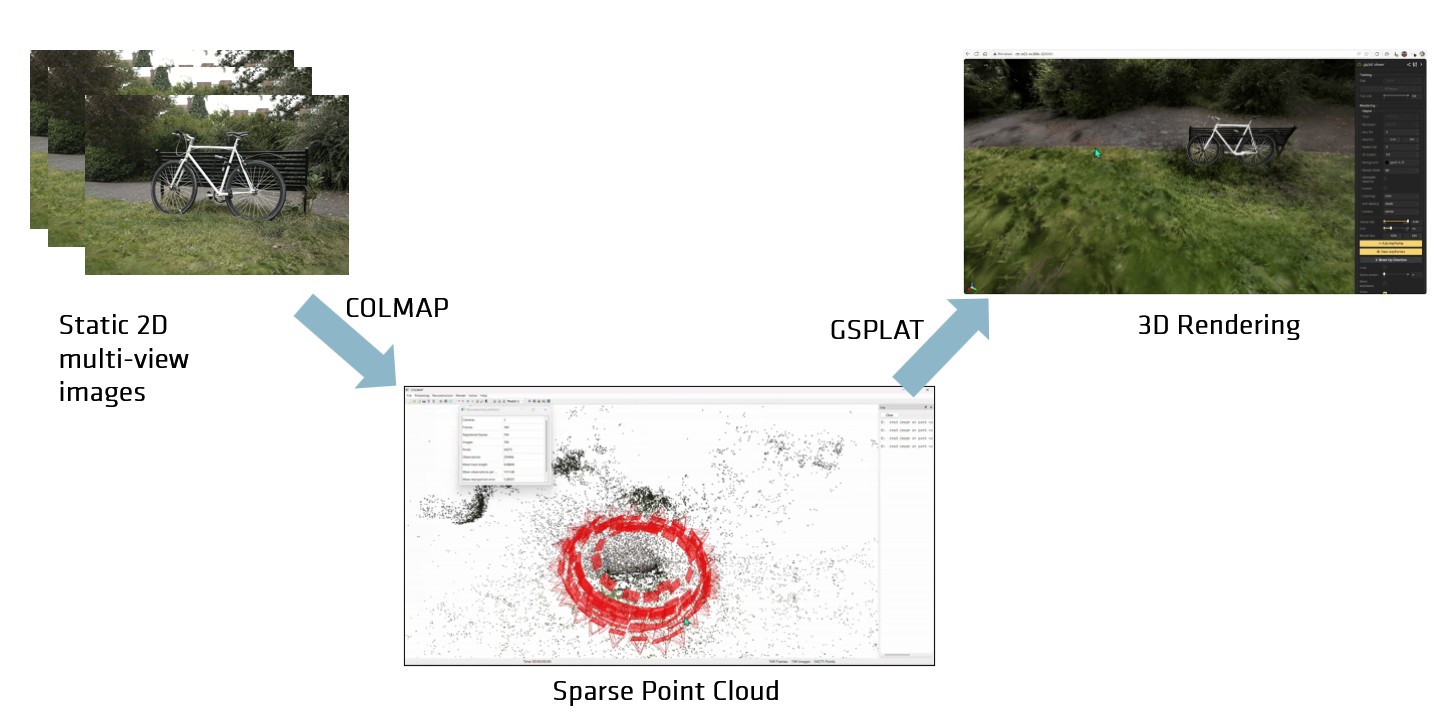
GSplat mapping and rendering process

The method then optimizes the parameters of the Gaussian primitives to reduce the discrepancy between the input images and the rendered outputs. The optimization typically employs a composite loss function combining L1 loss, which encourages pixel-wise accuracy, with the Structural Similarity Index Measure (SSIM) loss, which preserves perceptual image quality and structural consistency. During optimization, the gradients of the projected 2D Gaussian positions guide densification, while low opacity triggers the culling of Gaussians. Densification increases the number of Gaussians in underrepresented or visually inconsistent regions, using strategies such as splitting larger Gaussians into smaller ones or sampling new Gaussians where needed. Conversely, culling removes Gaussians that contribute minimally to the final rendered image, improving efficiency without sacrificing visual quality.

In summary, 3DGS combines the speed of explicit rendering, the flexibility of volumetric representation, and the ability to capture view-dependent appearance, offering a practical trade-off between rendering quality and computational efficiency.

Installing GSplat on AMD MI300X

System Requirements

GSplat for AMD ROCm™ 1.0.0 depends directly on PyTorch for AMD ROCm™

• ROCm: version 6.4.3 (recommended)

• Operating system: Ubuntu 22.04 and above

• GPU platform: AMD Instinct™ MI300X

• PyTorch: version 2.6 (ROCm-enabled) and above

Installation

Install PyTorch first. The easiest way is to use the official Docker image which has PyTorch for ROCm.

docker run --cap-add=SYS_PTRACE --ipc=host --privileged=true \
--shm-size=128GB --network=host --device=/dev/kfd --device=/dev/dri \
--group-add video -it -v $HOME:$HOME --name rocm_pytorch
rocm/pytorch:rocm6.4.3_ubuntu24.04_py3.12_pytorch_release_2.6.0

Install GSplat from the AMD hosted PYPI repository:

pip install gsplat --extra-index-url=https://pypi.amd.com/simple

Once the installation is successful, you can verify the installation using the pip show command:

pip show gsplat

Training GSplat on AMD MI300X

Now, it’s time to train the GSplat model using the prepared images of the scene. We run our experiments on AMD MI300X GPUs to ensure fast and efficient training. To demonstrate this we use the Mip-NERF 360 dataset which is a collection of four indoor and five outdoor object-centric scenes. The camera trajectory is an orbit around the object with fixed elevation and radius. The test set takes each n-th frame of the trajectory as test views.

You can download the dataset used in this tutorial from the GSplat GitHub repository using the steps below.

git clone --no-checkout https://github.com/rocm/gsplat.git  && cd gsplat && git sparse-checkout init --cone
git sparse-checkout add examples && git checkout main
cd examples
pip install -r examples/requirements.txt
python datasets/download_dataset.py

Once you have the dataset ready, you can use the command below to train a reconstructed 3D scene which is synthesized out of 2D images.

CUDA_VISIBLE_DEVICES=0 python simple_trainer.py default \
    --data_dir data/360_v2/bicycle/ --data_factor 4 \
    --result_dir ./results/bicycle

Rendering the scene

Now let’s put our newly reconstructed scene to the test by rendering some novel views!

You can use the splat viewer to view the reconstructed scene. The output of the training command above should show the URL of the splat Viser which can be connected via a web browser. The splat should appear something like this.

Exploring splat editing features

In addition to rendering existing scenes, GSplat also supports advanced features like splat editing. This allows users to manipulate existing datasets to introduce new elements seamlessly. You can use open source editing software like SuperSplat, which can be used for advanced operations like editing. You can drag and drop the splat file into the SuperSplat app, which will open up the 3D reconstruction with a host of options to perform more operations. The video below demonstrates how to add more objects from additional splat files into this scene and render it as a new scene. You can download the extra splat files from the HuggingFace repo VladKobranov/splats. After editing, you can see new objects added to the scene (a blue bicycle) and cropped the original bicycle scene.

Performance

GSplat supports multi-GPU training, delivering over 3× faster training and more than 3× lower memory usage per GPU. This is achieved through PyTorch’s Distributed Data Parallel (DDP) framework, which synchronizes and averages gradients across all GPUs.

You can use the command below for a multi-GPU based training.

CUDA_VISIBLE_DEVICES=0,1,2,3,4,5,6,7 python simple_trainer.py default  --data_dir data/360_v2/bicycle/ --data_factor 4  --result_dir ./results/bicycle 

The benchmark results clearly show that a distributed training system leads to a reduction in training time and memory usage per GPU rank. This is due to the independent training of Gaussians trained per GPU rank as shown in the graph below, which indicates the total training time, memory usage, and number of Gaussians per GPU rank for different distributed training scenarios.

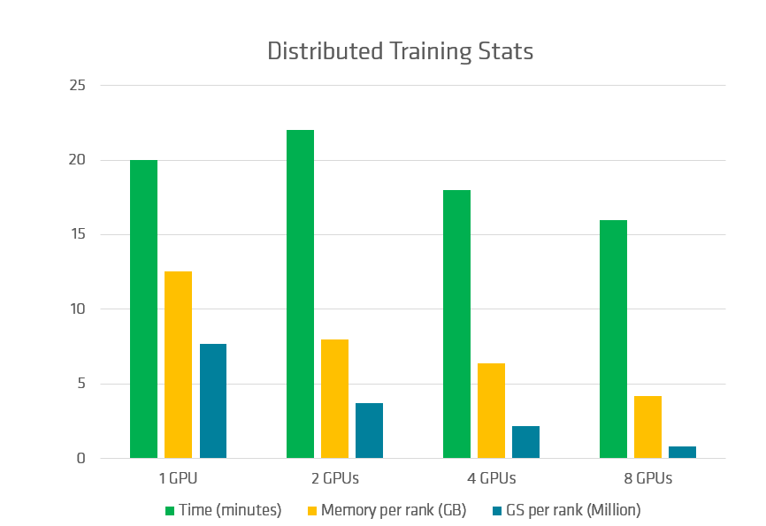
Distributed training benchmark results

Benchmarks

This repo comes with a standalone script that reproduces the official GSplat benchmarks with exactly the same performance on PSNR, SSIM, LPIPS, and converged number of Gaussians. Follow the below steps to run the evaluation:

cd examples
pip install -r requirements.txt
# download mipnerf_360 benchmark data
python datasets/download_dataset.py
# run batch evaluation
bash benchmarks/basic.sh

3DGS

The table below presents the consolidated average of evaluation metrics, training memory and time for a single GPU averaged over 6 scenes on the Mip-NERF 360 captures.

Configuration	PSNR	SSIM	LPIPS	Train Memory (GB)	Training Time (s)
gsplat-7K	27.61	0.83	0.16	4.81	158.38
gsplat-30K	29.16	0.87	0.10	6.89	888.77

Metric definitions

• PSNR (Peak Signal-to-Noise Ratio): This is the ratio between the maximum possible power of a signal and the power of corrupting noise. Higher values indicate better reconstruction quality. It is measured in decibels (dB), and typically values above 30dB represent good quality.

• SSIM (Structural Similarity Index): SSIM measures the similarity between two images by considering luminance, contrast, and structure. It ranges from -1 to 1, where 1 indicates perfect similarity. SSIM is more perceptually aligned than PSNR.

• LPIPS (Learned Perceptual Image Patch Similarity): LPIPS uses a neural network (here either AlexNet or VGG) to compute perceptual similarity between images. Lower values indicate more perceptually similar images. It’s considered to better align with human perception than PSNR or SSIM.

• The number of Gaussians and rendering time provide insights into model efficiency.

The below table shows the metrics, training time, and memory used during training for each scene.

Training Memory (GB)

Configuration	Bicycle	Bonsai	Counter	Garden	Kitchen	Room	Stump
gsplat-7k	6.70	2.85	2.82	7.26	3.04	2.81	6.16
gsplat-30k	11.59	2.95	2.82	11.06	3.59	3.61	8.56

Training Time (s)

Configuration	Bicycle	Bonsai	Counter	Garden	Kitchen	Room	Stump
gsplat-7k	147.44	161.15	169.35	168.50	175.19	155.99	142.11
gsplat-30k	1102.74	719.39	771.37	1067.28	814.53	758.39	870.30

PSNR

Configuration	Bicycle	Bonsai	Counter	Garden	Kitchen	Room	Stump
gsplat-7k	23.69	30.15	27.57	26.59	29.42	29.97	25.90
gsplat-30k	24.93	32.26	29.19	27.63	31.54	31.75	26.78

SSIM

Configuration	Bicycle	Bonsai	Counter	Garden	Kitchen	Room	Stump
gsplat-7k	0.67	0.93	0.89	0.83	0.91	0.90	0.73
gsplat-30k	0.76	0.94	0.91	0.87	0.93	0.92	0.77

LPIPS

Configuration	Bicycle	Bonsai	Counter	Garden	Kitchen	Room	Stump
gsplat-7k	0.30	0.13	0.18	0.11	0.11	0.19	0.23
gsplat-30k	0.16	0.11	0.13	0.07	0.08	0.14	0.14

Number of Gaussians

Configuration	Bicycle	Bonsai	Counter	Garden	Kitchen	Room	Stump
gsplat-7k	4.46M	1.55M	1.64M	4.83M	1.89M	1.48M	4.11M
gsplat-30k	7.78M	1.85M	1.30M	6.69M	2.12M	2.29M	5.73M

Summary

In this blog we walked through the basics of GSplat, exploring how to train a 3D Gaussian Splatting (3DGS) model and render novel views in real time. With features like multi-GPU support and experimental splat editing, GSplat makes it easier than ever to explore, tweak, and scale 3DGS workflows.

For installation instructions, API reference guides, and examples please have a look at the GSplat documentation page or view the source code on the ROCm GitHub repo.

In our next blog we will explore more advanced workflows, optimizations, and integrations with larger datasets. This is just the starting point — try it out, break things, and see what you can build!

Additional Resources

• Schonberger, Johannes L., and Jan-Michael Frahm. “Structure-from-motion revisited.” In Proceedings of the IEEE conference on computer vision and pattern recognition, pp. 4104-4113. 2016.

• Mildenhall, Ben, Pratul P. Srinivasan, Matthew Tancik, Jonathan T. Barron, Ravi Ramamoorthi, and Ren Ng. “Nerf: Representing scenes as neural radiance fields for view synthesis.” Communications of the ACM 65, no. 1 (2021).

• Kerbl, Bernhard, Georgios Kopanas, Thomas Leimkühler, and George Drettakis. “3D Gaussian splatting for real-time radiance field rendering.” ACM Trans. Graph. 42, no. 4 (2023): 139-1.

• Ye, Vickie, Ruilong Li, Justin Kerr, Matias Turkulainen, Brent Yi, Zhuoyang Pan, Otto Seiskari et al. “gsplat: An open-source library for Gaussian splatting.” Journal of Machine Learning Research 26, no. 34 (2025): 1-17.

Disclaimers

Third-party content is licensed to you directly by the third party that owns the content and is not licensed to you by AMD. ALL LINKED THIRD-PARTY CONTENT IS PROVIDED “AS IS” WITHOUT A WARRANTY OF ANY KIND. USE OF SUCH THIRD-PARTY CONTENT IS DONE AT YOUR SOLE DISCRETION AND UNDER NO CIRCUMSTANCES WILL AMD BE LIABLE TO YOU FOR ANY THIRD-PARTY CONTENT. YOU ASSUME ALL RISK AND ARE SOLELY RESPONSIBLE FOR ANY DAMAGES THAT MAY ARISE FROM YOUR USE OF THIRD-PARTY CONTENT.