Thread Trace Part 1: ROCprof Compute Viewer

September 15, 2026 by Giovanni Lenzi Baraldi, Gianpaolo Tommasi.

14 min read. | 3386 total words.

Software tools & optimizations

Profiling

Developers

Once you have identified a GPU kernel to optimize, you need to understand how its instructions execute and where waves spend time waiting. Thread trace gives you a detailed view of that behavior, helping you investigate stalls, gaps in execution, and competition for hardware resources.

In this first post of a three-part series on AMD GPU thread trace, you will learn to capture traces with rocprofv3 and analyze instruction timing, stalls, utilization, and performance counters in ROCprof Compute Viewer (RCV). You will follow a sample kernel from trace collection to analysis, connect source code to executed ISA instructions, and compare wave timelines with counter plots to investigate performance bottlenecks. These skills prepare you to explore the profiling APIs in Part 2 and advanced tracing workflows in Part 3.

Purpose of This Series

This is the first post in a three-part series that answers the following questions:

• What is thread trace, and when should you use it?

• What profiling information can and cannot be extracted from it?

• Which ROCm components are involved in an end-to-end thread trace workflow?

• How can profiling tool developers use the thread trace API?

• What are the common pitfalls when using thread trace?

• Part 1 demonstrates how to use rocprofv3 and RCV, a GUI for visualizing thread trace data.

• Part 2 focuses on the ROCprofiler SDK thread trace API and the ROCprof Trace Decoder API.

• Part 3 covers advanced thread trace features and workflows.

Audience and Requirements

Readers are expected to:

• Have a basic understanding of HIP applications and the ROCm software stack.

• Have read the introduction to profiling series and Occupancy basics.

This post is intended for kernel developers who want to optimize execution within a kernel and for third-party profiling tool developers who want to add thread trace support to their tools.

ROCm 7.13 or later is recommended. Thread trace support was introduced in ROCm 7.0, but releases earlier than ROCm 7.13 require you to build ROCprof Trace Decoder from source.

Hardware Support

GFXIP	ISA	Products	Support	Detailed trace scope
gfx908	AMD CDNA™ 1	AMD Instinct™ MI100 series	Partial	CU
gfx90a	AMD CDNA™ 2	AMD Instinct™ MI200 series	✔	CU
gfx942	AMD CDNA™ 3	AMD Instinct™ MI300 series	✔	CU
gfx950	AMD CDNA™ 4	AMD Instinct™ MI350 series	✔	CU
gfx1030	AMD RDNA™ 2	AMD Radeon™ RX 6000 series	Partial	SIMD
gfx1100	AMD RDNA™ 3	AMD Radeon™ RX 7000 series	✔	SIMD
gfx1150	AMD RDNA™ 3.5	Ryzen™ AI APUs	✔	SIMD
gfx1200	AMD RDNA™ 4	AMD Radeon™ RX 9000 series	✔	SIMD
gfx1250	AMD CDNA™ 5	AMD Instinct™ MI450 series	✔	SIMD

Getting the ROCprof Compute Viewer (RCV)

• Download prebuilt binaries from the ROCprof Compute Viewer releases page.

• Download bleeding-edge build artifacts from the most recent mainline build.

• To build RCV from source, follow the instructions in the ROCprof Compute Viewer README.

Terminology

Collecting and visualizing thread trace data involves several components and introduces several new concepts. The following dictionary provides a concise reference for common thread trace components, concepts, and acronyms.

Name	Expanded name	Description
Wave	Wavefront	A collection of lanes (HIP threads), usually in groups of 32, for example on AMD RDNA™, or 64, for example on MI300. It is sometimes called a warp. CPU analogy: Think of a CPU thread.
Lane	—	A single HIP thread within a wave. CPU analogy: Think of a lane in an AVX or SSE instruction.
SQ	SeQuencer	A hardware block responsible for scheduling waves and sending work to execution units such as VALU, SALU, and VMEM. It is located inside the compute unit.
SQTT	SeQuencer Thread Trace	An AMD GPU hardware feature capable of tracing the work sent to execution units, among other information, with near-cycle accuracy. It is sometimes called Shader Wave Trace or just Thread Trace.
ATT	Advanced Thread Trace	The rocprofv3 command-line implementation responsible for exposing the SQTT hardware feature to users. ATT is sometimes used interchangeably with SQTT.
ALU	Arithmetic Logic Unit	A hardware component responsible for processing mathematical operations.
SALU	Scalar ALU	A hardware component responsible for processing a single mathematical operation requested by the wave. CPU analogy: Think of a normal mathematical operation on the CPU.
VALU	Vector ALU	A hardware component responsible for batch processing mathematical operations requested by the wave. It executes 32 or 64 operations at a time. CPU analogy: Think of SSE or AVX instructions.
SMEM	Scalar Memory	A hardware component responsible for processing a single memory operation, normally for loading kernel arguments.
VMEM	Vector Memory	A hardware component responsible for batch processing memory operations in and out of VRAM, normally in groups of 32 or 64.
LDS	Local Data Share/Storage	A hardware component responsible for batch processing memory operations in and out of local memory. In CUDA/HIP terminology, this is the __shared__ declaration.
FLAT	flat_* or scratch_* instruction	For SQTT on MI300, global_* memory operations are considered flat in the sense of the flat address space, even though they follow VMEM rules.
MSG	Message	An instruction that uses the message bus to signal other waves in a workgroup or components external to the CU. For example, instructions in __syncthreads() use it: s_barrier and s_barrier_signal.
IMMED	Internal instruction	An instruction that is not sent to an execution unit. It is internal to the wave and does not directly stall a pipe or other waves. Examples include s_sleep (sleep for a specified number of cycles), s_nop (do nothing), s_waitcnt (wait for a memory operation to complete), and s_barrier_wait (wait for other threads to arrive at __syncthreads()).
JUMP	Branch taken	A token indicating that a branch was taken.
NEXT	Branch not taken	A token indicating that a branch was not taken.
ISA	Instruction Set Architecture	A list of basic operations that can be performed by a program. It lies below source abstractions such as C++.
Slot	Wave ID or wave slot	A hardware unit capable of holding a wave. CPU analogy: Think of a CPU core with SMT as a two-slot core that can schedule two threads.
SIMD	Single Instruction, Multiple Data (unit)	A hardware unit containing multiple slots that can execute work independently from other SIMDs. A SIMD typically contains 8 or 16 wave slots. Most often, a SIMD can execute only one instruction of each type per (quad)cycle. In practice, one of the 8 or 16 waves inside the SIMD is selected to execute during that (quad)cycle. CPU analogy: This is closest to a heavily multithreaded CPU core.
CU	Compute Unit	A hardware unit containing four SIMDs and one LDS space. A workgroup (thread block) is contained within a single CU. A CU can sometimes contain two SIMDs depending on definition, but this detail is omitted here for simplicity.
WGP	Workgroup Processor	A hardware unit containing four SIMDs and one LDS space. It is used interchangeably with CU in this post for simplicity, even though the WGP-to-CU ratio can be 2:1.
SE	Shader Engine	A hardware unit containing multiple compute units for the purposes of this post.
—	Kernel dispatch	The command for the GPU to launch waves on the hardware and execute code in functions declared with __global__.
—	SQTT performance monitor	An MI200-series and MI300-series hardware feature capable of polling and updating selected SQ counters at < 100 nanosecond intervals. Do not confuse it with PMC or SPM, which also use hardware counters through different mechanisms.
SPM	Streaming Performance Monitor	A mechanism that collects hardware counters quickly and streams them into a buffer.

Note

For simplicity, this post sometimes uses the name of a hardware unit for the instructions sent to that unit. For example, a “VALU instruction” means an instruction that sends work to the VALU. This shorthand has limits because an instruction can use different hardware paths under different circumstances.

Note

The MI200 and MI300 series issue instructions at a quadcycle rate: the minimum issue interval is four cycles, so SQTT timing on these devices is a multiple of four cycles. On gfx10 and later architectures, including AMD RDNA™ and MI450, the issue rate is one cycle. This post uses “(quad)cycle” to mean the appropriate issue rate for each architecture.

Component name	Description
ROCprofiler SDK	A ROCm library for extracting profiling information from AMD GPUs, including SQTT data.
rocprofv3	A command-line tool that profiles ROCm applications by using the ROCprofiler SDK API.
ROCprof Trace Decoder	A ROCm library that decodes and interprets the hardware-defined SQTT data format and exposes it in a form that tools can consume.
ROCprof Compute Viewer (RCV)	A GUI for visualizing thread trace data. Do not confuse it with ROCm Compute Profiler (rocprof-compute), the application and kernel profiler built on ROCprofiler SDK.

What is Thread Trace and When Should I Use It?

Thread trace, or SQTT, is a near-cycle-accurate capability built into AMD GPU hardware. It records the math, memory, control-flow, and synchronization instructions executed by selected waves on the device. Depending on the architecture and instruction type, a traced instruction can provide:

• The clock cycle when it was issued.

• The time it stalled after the wave was ready to issue the instruction but the required pipeline could not accept it.

• The time required to complete execution after issue.

• The time the wave was idle because it was not ready to attempt another instruction.

Together, these events form a cycle-by-cycle time series of wave scheduling, instruction issue, and stalls. This detail produces a large amount of data in a short time, which leads to two practical limitations:

• Detailed instruction tracing is limited to a target CU or SIMD, depending on the architecture.

• Thread trace is not the first tool for surveying an application that runs for minutes or hours. First use a broader method, such as system tracing, dispatch counter collection, or PC sampling, to identify a small set of kernels for deeper analysis.

Note

The compute unit being traced is called the target CU. Thread trace operates independently in each shader engine, so the single-target-CU limitation applies per shader engine. For example, a GPU with 32 shader engines can trace 32 independent target CUs at the same time, although this is not recommended because of the memory-bandwidth requirements.

Note

Triple buffering can collect thread trace for an unlimited amount of time. A later post in this series will cover that advanced workflow.

At a surface level, thread trace contains two main categories of information:

• Detailed events provide the instruction-level trace. They are limited to a target CU on the AMD Instinct™ MI200, MI300, and MI350 series, or a target SIMD on AMD RDNA™ and AMD Instinct™ MI450 series.

• Global events are visible across a shader engine. Examples include wave start and end times, SQTT perfmon samples, instrumentation markers, kernel dispatches, and cache-flush events.

Your First Thread Trace With Rocprofv3 ATT and RCV

Setup

For the first example, use the provided phases.cpp application, which contains a kernel with several distinct activity phases. Compile and test the application:

# -g adds the debug information used for source correlation in RCV.
hipcc -g src/phases.cpp -o phases
./phases

Profiling

Now, profile with rocprofv3 ATT:

rocprofv3 --att --kernel-include-regex phases -d outdir -- ./phases

Parameter Name	Description
--att	Enables thread trace.
--kernel-include-regex phases	Traces only kernel names that contain the word phases.
-d outdir	Writes profiler output to a directory named outdir.

See the rocprofv3 thread trace documentation for the complete parameter list.

After profiling completes, outdir contains three types of output:

• A stats_*.csv file with a summary of instruction latencies observed for the traced waves.

• One ui_output_agent_{N}_dispatch_{M} directory for each traced kernel:

  • N identifies the GPU agent.

  • M identifies the dispatch sequence number observed by the profiler.

  • You can match agent and dispatch IDs to data collected with --kernel-trace --output-format csv.

  • The directory contains decoded thread trace data in JSON format and source snapshots for visualization.

• A {hostname} directory containing undecoded trace data and any non-ATT profiler output.

Opening a Trace in RCV

The item of interest is the ui_output_agent_{N}_dispatch_{M} directory. If you profiled on a remote machine, compress and copy this directory to your local machine. sshfs also works, but it can be slow for large traces. Open the directory in either of these ways:

• From the command line: ./rocprof-compute-viewer /path/to/ui/directory

• From the viewer: Import > rocprofv3 UI Output, as shown in Figure 1.

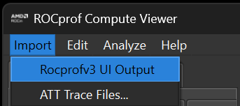
Figure 1. Importing a rocprofv3 UI output directory.

Instructions and Trace Tokens

Note

For AMD RDNA™ and AMD Instinct™ MI450 users, the trace looks different, but the same qualitative analysis workflow applies.

Left side: Input tab

Use the Input tab in Figure 2 to select the target wave and adjust the timeline range. The controls below determine which events you inspect in the other views.

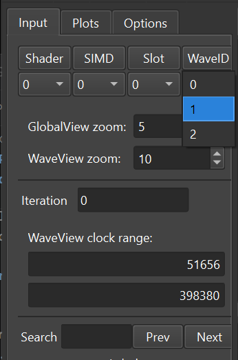
Figure 2. Input tab.

• Shader Engine, SIMD, Slot, and WID select the target wave. The target wave determines:

  • Which thread trace token RCV scrolls to when you click an ISA instruction.

  • Which wave defines loop iteration counts.

  • Which wave RCV uses to visualize branch targets.

• WaveView Clock Range selects the cycle window used by the Compute Unit, Utilization, and Hotspot views.

• WaveView zoom and GlobalView zoom control the local and global timeline scales.

• Search jumps to instructions such as ds_*, global_*, flat_*, or s_waitcnt, while History returns to previously selected tokens.

The Options tab contains miscellaneous viewer settings. The Plots tab is discussed in Visualizing counters.

Source and ISA View

The Source and ISA view connects source code, disassembled ISA, and the dynamic events in the timeline. Figure 3 shows how this view places instruction costs alongside the source and ISA lines. It shows every ISA instruction with hit-count and cost columns. Compile with hipcc -g before collecting a trace if you want source correlation. With debug information present, RCV can map ISA instructions to source lines. Hovering over or clicking an ISA line highlights the corresponding source line. Clicking a source line pins its ISA instructions until you select another line.

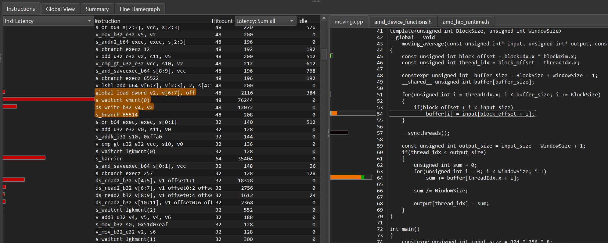
Figure 3. Aggregate latency by source and ISA line. Hovering over or clicking a source line highlights the corresponding ISA instructions. See the Compute Unit section for the color coding.

Hovering over an instruction can also reveal its inline source call stack. Figure 4 shows this context for a synchronization instruction associated with __syncthreads().

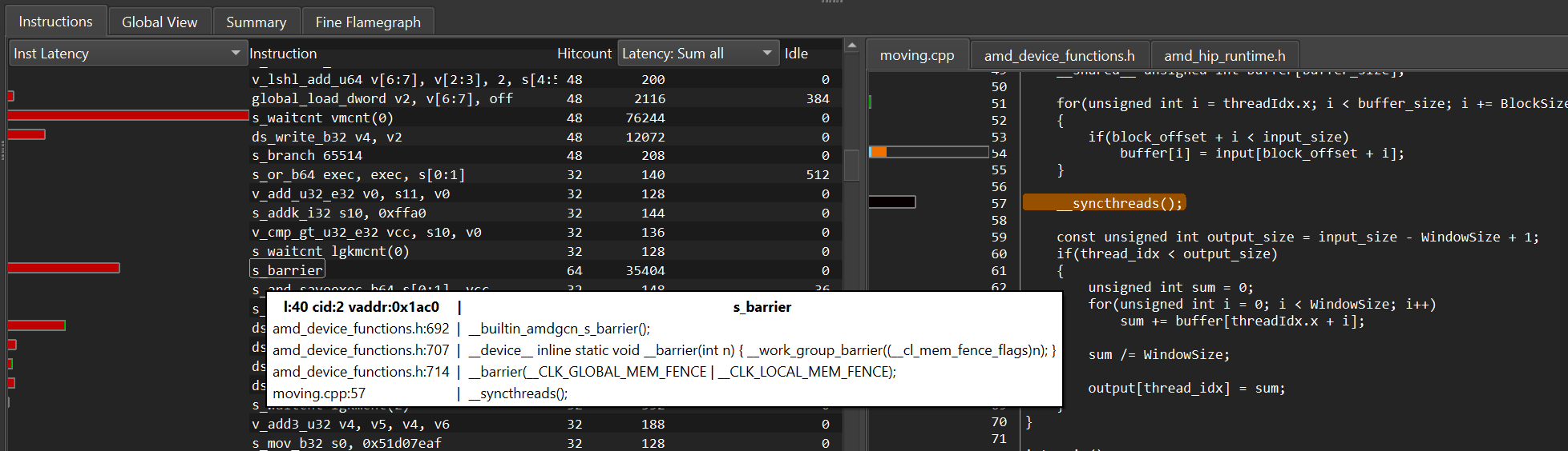
Figure 4. Inline call stack for __syncthreads(), displayed by hovering over the instruction.

Note

Treat this as a compiler-generated mapping, not a one-to-one source statement view. Optimized kernels often map one source line to many ISA instructions, inline functions can produce source stacks, and some ISA instructions might not have a useful source reference.

s_waitcnt Dependencies

Figure 5 shows how dependency arrows connect the scalar loads that fetch kernel arguments to the s_waitcnt instruction that waits for those loads to complete.

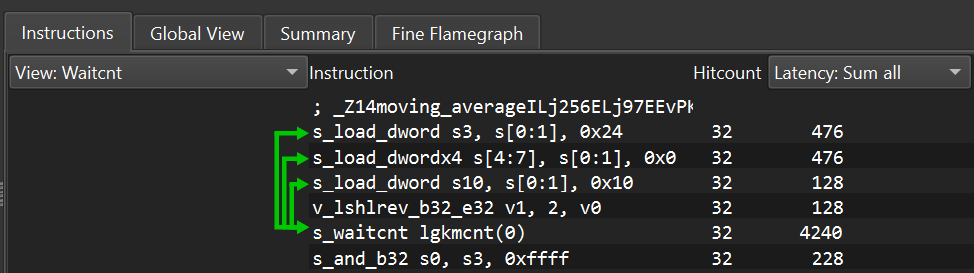
Figure 5. s_load_* instructions loading kernel arguments, followed by an s_waitcnt instruction that waits for them.

AMD GPU memory operations are asynchronous from the wave’s point of view. After issuing a memory operation, the wave can continue issuing independent instructions and wait for the memory operation later with an s_waitcnt or s_wait_* instruction. View: Waitcnt draws arrows from memory-producing instructions to the wait instruction that depends on them. Unlike static analysis, which is generally limited to basic blocks, thread trace can dynamically track wait dependencies per wave across branches and long jumps.

Branch Targets

Figure 6 shows a backward branch produced by a C++ loop, illustrating how the ISA view helps you follow repeated execution.

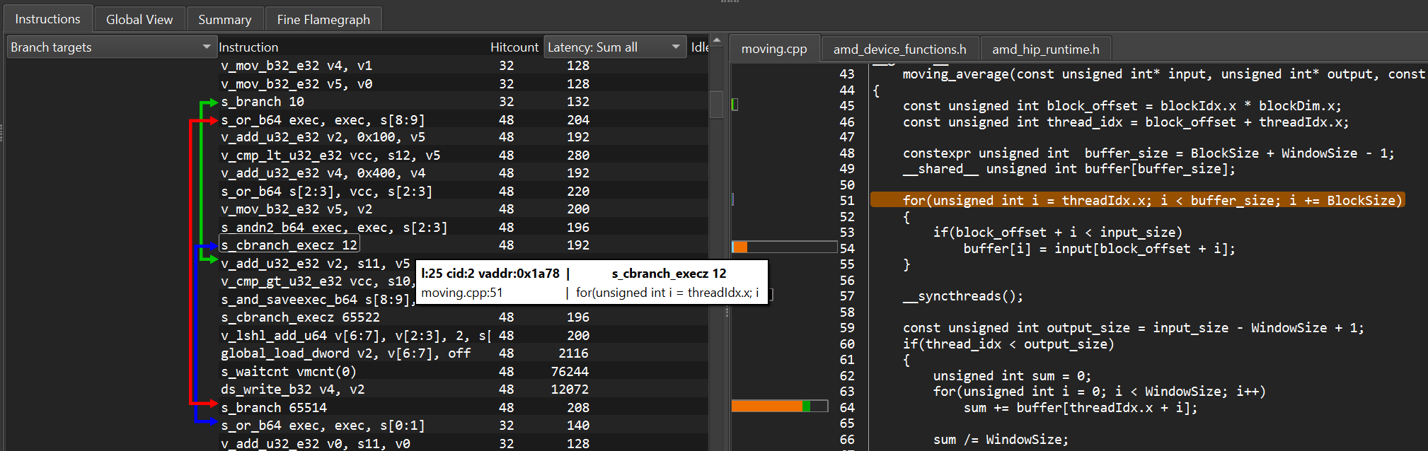
Figure 6. Branch target produced by a C++ loop.

The Branch targets mode draws the observed control-flow targets for branch and jump instructions in the selected wave. Backward arrows usually indicate loops, while forward arrows often indicate skipped blocks or exits from conditionals. Branches not executed or not taken are not drawn.

Hotspot and Fine Flamegraph

The Hotspot tab displays a histogram of instruction costs in cycles. RCV computes it over all waves inside the current WaveView Clock Range, not only the target wave. Changing the visible cycle range therefore changes the histogram. Clicking a bin highlights the first and last ISA lines represented in that cost range.

Idle time is not included in the hotspot calculation; only execution and stall cost are counted. The histogram is therefore useful for identifying expensive instructions, but it does not directly explain gaps where no wave issues. IMMED instructions such as s_waitcnt, s_barrier, and s_nop can appear expensive because many waves can wait at similar instructions concurrently.

The Fine Flamegraph rolls the same instruction cost up through the available source, inline, marker, and ISA hierarchy. Use it to answer “Which source region accounts for the most traced cost?” rather than “Which single ISA line is expensive?” When SQTT instrumentation markers are present, marker scopes provide another grouping layer around the source and ISA cost.

Latency

The Latency selector changes how RCV summarizes the instruction cost column. Latency: Sum all and Latency: Mean all aggregate across all traced waves in the current data set. Latency: Sum Wave, Latency: Mean Wave, and Latency: Max Wave focus on the target wave. Latency: Iteration shows the selected loop iteration for the current target wave. Use sum modes to find total cost, mean modes to find typical per-hit cost, and max or iteration modes to inspect outliers.

The Idle column is separate from instruction latency. It represents cycles between instructions during which the wave was not issuing and the relevant pipeline was not busy.

RCV can also show the percentage of an instruction’s latency that overlapped other useful work. For simplicity, this hidden-latency value includes hidden idle time rather than reporting it separately. Flamegraphs can display either total latency or only non-hidden latency. Figure 7 shows the latter view, helping you locate source regions whose latency other work did not hide.

Figure 7. Flamegraph display weighted by non-hidden latency.

Note

The current hidden-latency calculation uses a simplified priority order based on instruction type: WMMA > VALU > VMEM/LDS/FLAT > SMEM/SALU > OTHERS. For example, VALU execution can hide VMEM latency but not WMMA latency. RCV runs this analysis automatically for gfx10 and later traces; you can also run it manually for gfx9 from Analyze > Hidden Latency.

Compute Unit and Utilization

Waves Competing for Resources

Several active waves can reside in a SIMD, each occupying a wave slot and sharing the unit’s issue and execution resources. Depending on the architecture, multiple waves can issue work to different pipelines in the same (quad)cycle, while waves that need the same pipeline compete for it. When wave A waits on an s_waitcnt instruction or a barrier, the scheduler can often select a ready wave B, hiding some or all of wave A’s latency. RCV summarizes this latency-hiding behavior in aggregate, while the cycle-by-cycle view complements that summary by showing how instruction issue and stalls evolve over time.

The Compute Unit tab separates the detailed trace by SIMD and slot. Each row is a wave slot, and each colored token represents an instruction or event from a wave occupying that slot. Left-clicking a token highlights the corresponding ISA line. Right-clicking and dragging measures cycles. The A and D keys pan horizontally, while WaveView zoom or Ctrl + mouse wheel changes the timeline scale.

In the Compute Unit timeline, stall means that the wave is ready to issue an instruction, but the required pipeline cannot accept it. Idle means that the wave is not ready to attempt another instruction. This distinction helps separate pipeline contention from periods when the wave has no instruction ready to issue.

RCV uses a consistent color scheme to distinguish token types such as VMEM, VALU, LDS, scalar, message, and immediate instructions. Figure 8 shows the color assigned to each token category.

Figure 8. Color legend for instruction and token types in RCV.

At a wider zoom level, the Compute Unit view shows the general reason for activity in each wave over time, as illustrated in Figure 9. This view helps compare wave behavior and identify broad activity phases before zooming in to inspect individual instructions.

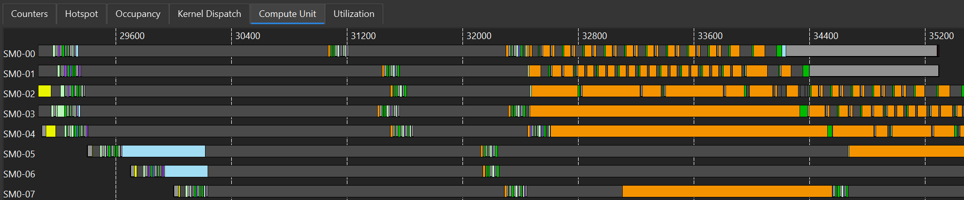
Figure 9. Zoomed-out Compute Unit view showing the general reason for activity in each wave.

The Utilization tab aggregates the same local trace by instruction type, such as VALU, VMEM, LDS, SCALAR, and OTHER. It hides IMMED tokens because multiple waves can process them in parallel, and it hides stalled time so the view emphasizes active issue and execution resources. Empty regions in Utilization are useful bubble candidates, but compare them with the Compute Unit rows to determine whether waves were absent, stalled, or executing an instruction type hidden by the view. Ctrl + left click keeps multiple top-level tabs open at the same time.

Figure 10 places the Compute Unit and Utilization timelines together so you can relate gaps in VALU execution to waves trying to issue SALU instructions or waiting on memory.

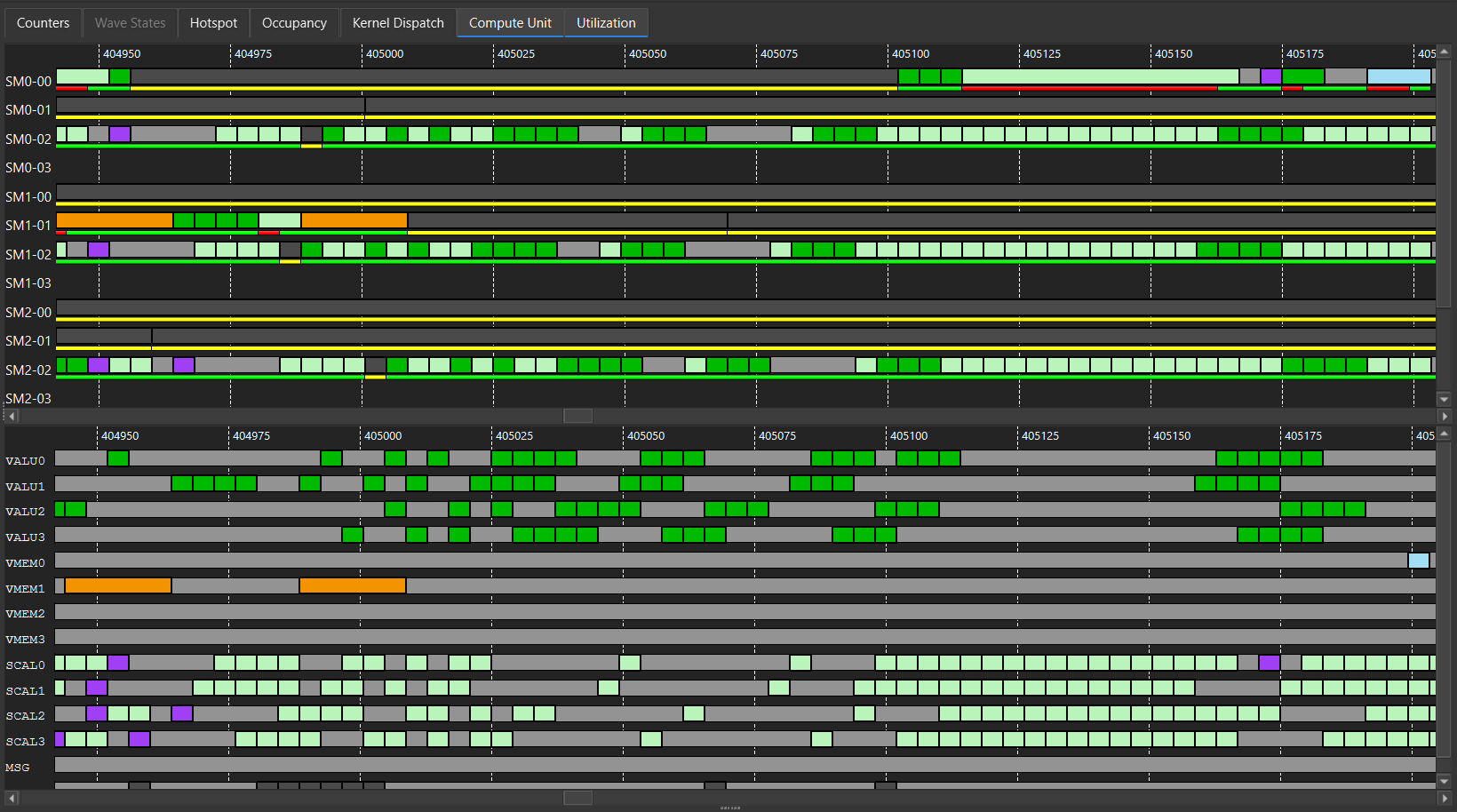
Figure 10. Zoomed-in Compute Unit and Utilization views. In this example, bubbles appear in VALU execution while all waves are either trying to issue SALU instructions or waiting on memory.

Loop Navigation

The Iteration box is the easiest way to inspect repeated executions of the same instruction. Clicking a token updates the selected ISA line and iteration number. Editing the iteration number scrolls the Compute Unit and Utilization timelines to another execution of the same instruction for the target wave, starting at iteration zero.

FIFO: An Example of Issue-stall Behavior

Figure 11 illustrates an LDS issue stall caused by FIFO backpressure, representing the trace as seen by a single wave:

Figure 11. Stall due to FIFO full.

The first several LDS instructions (orange) issue quickly and are followed by a long stall. SQTT records when these instructions issue, not when the memory operations complete. The operations continue in the background, and the wave normally synchronizes with them later through an s_waitcnt. When the request FIFO becomes full, backpressure stalls the next LDS instruction that attempts to issue.

LDS and VMEM completion behavior can be tracked with SQTT perfmon or SPM counters. In particular, FIFO-level counters can help confirm this kind of backpressure. The Visualizing counters section demonstrates this workflow.

Other SIMD Activity on AMD RDNA™ and AMD CDNA™ 5

AMD RDNA™ and AMD CDNA™ 5 provide detailed tracing for one SIMD at a time, with one exception: SQTT also records VMEM and LDS instruction issue from the other SIMD that shares the same VMEM/LDS unit. This information helps you track memory-pipeline utilization across the pair of SIMDs, even though only the target SIMD has a full detailed trace.

Visualizing Counters

rocprofv3 provides several methods for collecting performance counters alongside thread trace. This section covers two methods: SQTT perfmons and the Streaming Performance Monitor (SPM).

Note

SQTT perfmons are available on the MI200 and MI300 series, with partial support for other gfx9-based products. gfx9 products can also use SPM. On gfx10 and later products, only SPM is available, and it is improved to cover the use cases served by both methods.

SQTT perfmons stream SQ counters directly into the trace. SPM uses a separate buffer for independent collection, which is later matched with the trace. The following table compares them:

Characteristic	SQTT perfmon	SPM
Spatial granularity for SQ counters	Compute unit	Shader engine
Typical stable polling rate	~120 clocks	~4,000 clocks
Correlation with thread trace	Accurate	Approximate
Bandwidth use at maximum polling rate	High	Medium
Counter variety	Low: SQ only	High: SQ, TCP, TCC, TCA, and others
Supports per-SIMD counters	✔	X

In short, SQTT perfmons support faster counter collection, while SPM provides a richer counter set and can, for example, show cache hit rates.

Collecting SQTT Perfmons

Parameter	Description
--att-perfcounter-ctrl	Sets the sampling interval. A value of 1 is the fastest setting: approximately 40 cycles for up to four counters and approximately 80 cycles for more than eight counters.
--att-perfcounters	Specifies the SQ counters to collect.
--att-activity	Shorthand for --att-perfcounters and --att-perfcounter-ctrl. It collects a predefined set of counters for displaying general activity at the specified sampling period.
--att-perfcounter-target-only	Restricts counter collection to the target CU, substantially reducing bandwidth. This setting is recommended.

The recommended first use is:

rocprofv3 --att-activity 8

Figure 12 shows the activity counters as derived counter plots aligned with the thread trace, allowing you to compare counter values with instruction activity over time.

Figure 12. Activity counters displayed as derived counter plots.

An example to track LDS and VMEM FIFO depth at the target CU:

rocprofv3 --att-perfcounter-ctrl 1 --att-perfcounters "SQ_INST_LEVEL_LDS SQ_INST_LEVEL_VMEM" --att-perfcounter-target-only 1

An example to track bank conflicts across each SIMD:

rocprofv3 --att-perfcounter-ctrl 1 --att-perfcounters "SQ_LDS_BANK_CONFLICT:1 SQ_LDS_BANK_CONFLICT:2 SQ_LDS_BANK_CONFLICT:4 SQ_LDS_BANK_CONFLICT:8" --att-perfcounter-target-only 1

Note

The : syntax defines the SIMD mask for each counter. For example, SQ_LDS_BANK_CONFLICT:0xF enables all four SIMDs, which is the default, while SQ_LDS_BANK_CONFLICT:2 enables only SIMD 1 because 2 = 1 << 1.

Figure 13 shows how FIFO-depth and bank-conflict plots let you compare outstanding memory work with LDS bank conflicts over time. This example aggregates counters across all CUs; the commands above restrict collection to the target CU.

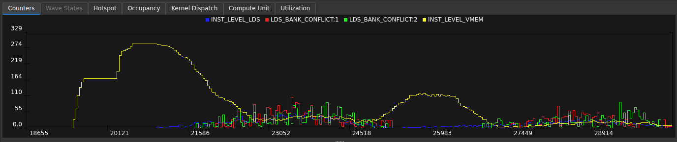
Figure 13. VMEM and LDS FIFO depth with LDS bank-conflict counters for SIMD 0 and SIMD 1, aggregated across all CUs.

Collecting Basic Counters with SPM

Streaming Performance Monitors can be collected alongside thread trace. See the RCV SPM guide for more information. For example:

rocprofv3 --att --spm SQ_CYCLES TCC_HIT TCC_MISS TA_TA_BUSY TCP_TOTAL_CACHE_ACCESSES TCP_TCC_WRITE_REQ TCP_TCC_READ_REQ -d test --spm-beta-enabled 1 --spm-sample-interval-unit sclk_cycles --spm-sample-interval 4096 --kernel-include-regex mykernel -f json -- ./a.out

Keep these requirements in mind:

• SQ_CYCLES must be collected for clock alignment with thread trace.

• -f json is mandatory because only JSON output is currently supported.

• Defining --kernel-include-regex and --kernel-iteration-range is highly recommended because SPM outputs to a single JSON file.

Derived Counters

RCV lets you define and edit derived counters in real time. Select Edit > Derived Counters > + New to create a derived counter file. Derived counters work with both SPM and SQTT perfmon samples.

When you use --att-activity, RCV provides an initial set of definitions when you create a derived counter file. Select Help in the editor for the complete expression syntax. The Plots menu in the left panel displays counter values and provides checkboxes for showing or hiding individual plots.

Figure 14 uses a kernel designed to show how SPM samples align with thread trace. The kernel contains five phases, distinguished by the dominant trace colors:

1. Light gray, left: poorly coalesced memory accesses, with low L1 efficiency and bandwidth and high L1/L2 miss rates.

2. Green, near cycle 153600: high VALU utilization with no cache activity.

3. Dark gray, near cycle 256000: well-coalesced memory accesses with high L1 efficiency but low L1/L2 hit rates.

4. Green and orange: mixed VALU, LDS, and memory operations.

5. Cyan, near cycle 665600: high L1 hit rate, efficiency, and bandwidth.

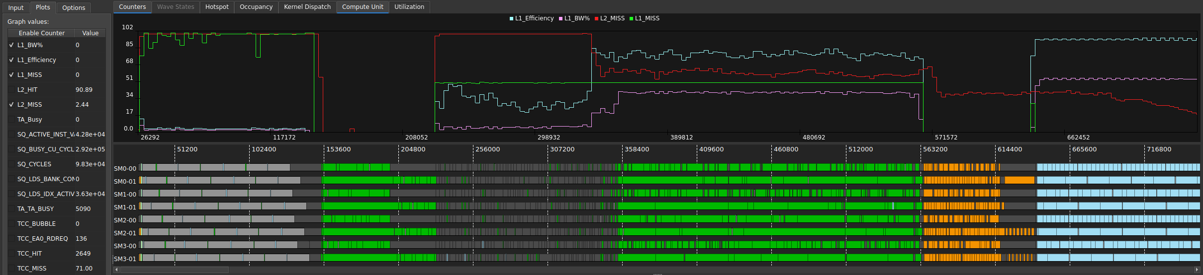
Figure 14. Kernel designed to show SPM derived counters aligned with the trace.

The following sample derived-counter file selects XCC 0, SE 0, and CU 1. RCV treats variables whose names start with an underscore as temporary values and does not plot them. These variables can be used for intermediate calculations.

_cycles := max[select[select[SQ_CYCLES, 0, axis=XCC], 0, axis=SE], axis=CU] + 0.001

_L2_HIT := sum[select[select[TCC_HIT, 0, axis=XCC], 0, axis=SE], axis=CU]
_L2_MISS := sum[select[select[TCC_MISS, 0, axis=XCC], 0, axis=SE], axis=CU]

_TA_BUSY := select[select[select[TA_TA_BUSY, 0, axis=XCC], 0, axis=SE], 1, axis=CU]
_TCP_TOTAL := select[select[select[TCP_TOTAL_CACHE_ACCESSES, 0, axis=XCC], 0, axis=SE], 1, axis=CU]
_TCP_WRITE := select[select[select[TCP_TCC_WRITE_REQ, 0, axis=XCC], 0, axis=SE], 1, axis=CU]
_TCP_READ := select[select[select[TCP_TCC_READ_REQ, 0, axis=XCC], 0, axis=SE], 1, axis=CU]

L2_MISS := 100 * _L2_MISS / (_L2_HIT + _L2_MISS + 30)
L1_MISS := 100 * min((_TCP_READ + _TCP_WRITE) / (_TCP_TOTAL + 1), 1)

TA_Busy := 100 * _TA_BUSY / _cycles
L1_BW% := 50 * _TCP_TOTAL / _cycles

L1_Efficiency := 100 * min(_TCP_TOTAL, _TA_BUSY) / max(_TA_BUSY, 10)

Summary

In this blog, you learned how to collect thread trace data with rocprofv3 and analyze it in ROCprof Compute Viewer. RCV connects source code and ISA with instruction timing, branch and wait dependencies, wave activity, stalls, and hardware counter data. These views help identify expensive instructions, execution bubbles, memory backpressure, and latency hidden by other work. Thread trace is most useful after broader profiling has identified a kernel for detailed analysis. Part 2 of this series will cover collecting and decoding thread trace data through the ROCprofiler SDK and ROCprof Trace Decoder APIs.

Disclaimers

The information presented in this document is for informational purposes only and may contain technical inaccuracies, omissions, and typographical errors. The information contained herein is subject to change and may be rendered inaccurate for many reasons, including but not limited to product and roadmap changes, component and motherboard version changes, new model and/or product releases, product differences between differing manufacturers, software changes, BIOS flashes, firmware upgrades, or the like. Any computer system has risks of security vulnerabilities that cannot be completely prevented or mitigated. AMD assumes no obligation to update or otherwise correct or revise this information. However, AMD reserves the right to revise this information and to make changes from time to time to the content hereof without obligation of AMD to notify any person of such revisions or changes. THIS INFORMATION IS PROVIDED “AS IS”. AMD MAKES NO REPRESENTATIONS OR WARRANTIES WITH RESPECT TO THE CONTENTS HEREOF AND ASSUMES NO RESPONSIBILITY FOR ANY INACCURACIES, ERRORS, OR OMISSIONS THAT MAY APPEAR IN THIS INFORMATION. AMD SPECIFICALLY DISCLAIMS ANY IMPLIED WARRANTIES OF NON-INFRINGEMENT, MERCHANTABILITY, OR FITNESS FOR ANY PARTICULAR PURPOSE. IN NO EVENT WILL AMD BE LIABLE TO ANY PERSON FOR ANY RELIANCE, DIRECT, INDIRECT, SPECIAL, OR OTHER CONSEQUENTIAL DAMAGES ARISING FROM THE USE OF ANY INFORMATION CONTAINED HEREIN, EVEN IF AMD IS EXPRESSLY ADVISED OF THE POSSIBILITY OF SUCH DAMAGES. AMD, the AMD Arrow logo, and combinations thereof are trademarks of Advanced Micro Devices, Inc. Other product names used in this publication are for identification purposes only and may be trademarks of their respective companies. © 2026 Advanced Micro Devices, Inc. All rights reserved.