HPC Coding Agent - Part 3: MCP Tool for Profiling#

In this blog, we build an AI agent specialized in profiling and optimizing GPU-accelerated applications within High-Performance Computing (HPC) environments. Using open-source tools, we create a state-of-the-art agent and enhance its profiling capabilities through a custom Model Context Protocol (MCP) server. This server provides the agent with tools to leverage AMD’s profiling utilities for analyzing application performance on AMD GPUs.
High-performance computing is expensive in capital investment and energy. When workloads run for hours or days, every inefficiency multiplies into wasted resources and delayed insights. Optimizing application performance is essential for making HPC both sustainable and cost-effective.
Effective optimization of GPU-accelerated applications requires a deep understanding of both hardware architecture and profiling tools. While a variety of tools exist for profiling execution time, memory usage, and other performance metrics, they present challenges for AI agents. These tools typically offer extensive configuration options, produce output in formats designed for human interpretation (large database files, natural language descriptions, or graphs), and require domain expertise to use effectively. By creating an MCP server that provides simplified interfaces and machine-readable output, we can significantly enhance an AI agent’s ability to leverage these profiling tools for automated performance optimization.
We’ll show how to set up the agent step-by-step and use it to profile and optimize an example application, comparing the agent’s performance against that of an experienced human profiler.
This blog is the third installment in our series on enhancing AI agent capabilities in HPC environments. For an introduction to the topic, including how to improve an agent’s HPC domain understanding, see Part 1: Combining GLM-powered Cline and RAG Using MCP. And to learn about effective code optimization using evolutionary algorithms, see Part 2: An MCP Tool for Code Optimization with OpenEvolve.
Architecture#
The architecture (Figure 1) combines three main components, GLM-4.6, Cline and our MCP Profiling Server, to enable AI-assisted profiling and optimization of HPC workloads:
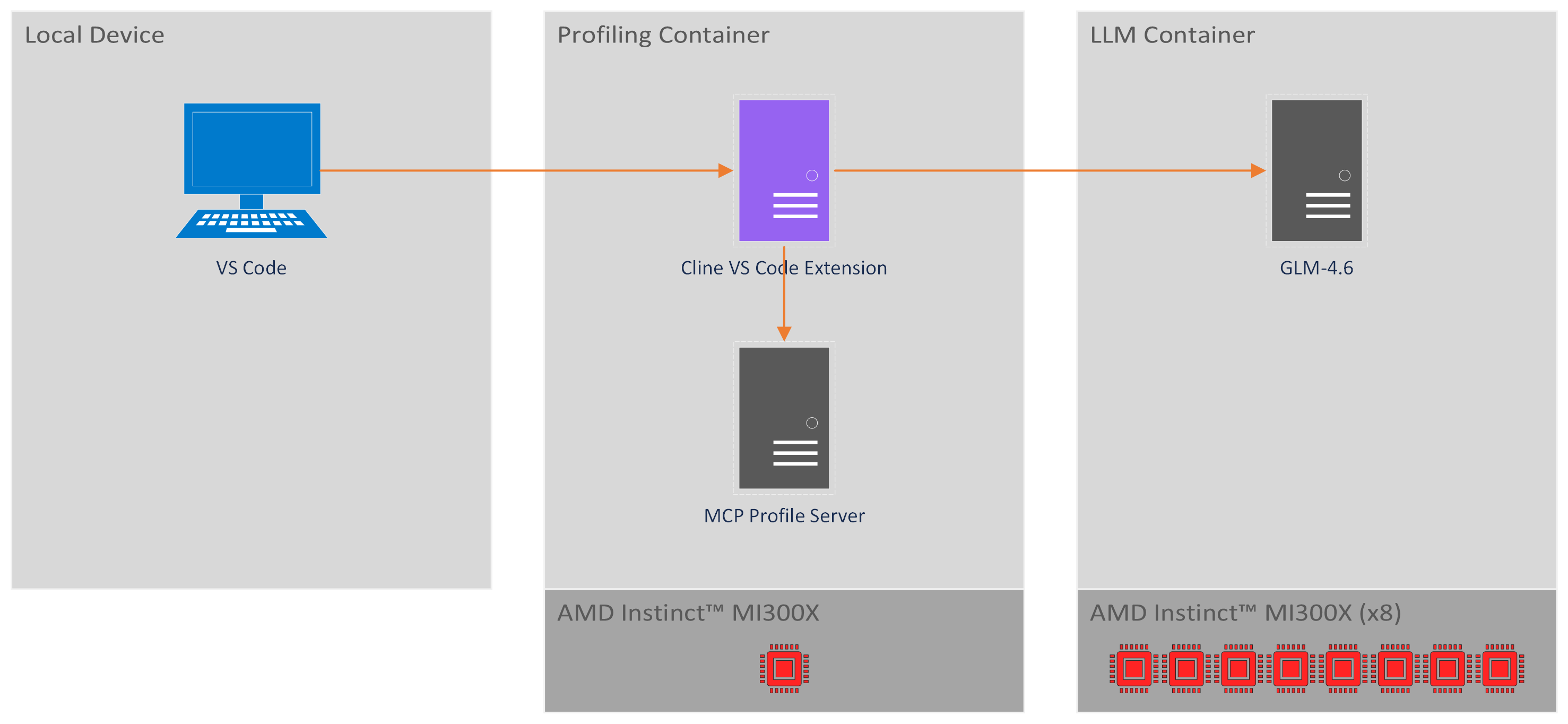
Figure 1. Architecture diagram of the HPC coding agent with MCP tools for profiling.#
GLM-4.6:
An open-source LLM that powers the coding agent’s intelligence with 355B parameters and a 200K token context window. For more details, see GLM-4.6.
The GLM-4.6 model runs in a dedicated container that utilizes all eight AMD Instinct™ MI300X GPUs on our node. While a lighter setup can operate with four GPUs, this configuration limits the LLM’s capabilities, reducing the context window from 200K to 50K tokens.
Cline:
An open-source AI coding agent that interacts with the LLM and executes tasks through planning and acting modes. It can generate code, edit files, and use command-line tools. It is provided as a Visual Studio Code (VS Code) extension, but can also be used through a CLI version with the same functionality but without a GUI. For more details, see Cline.
Cline operates within a dedicated profiling container, which also serves as the execution environment for profiling and optimization tasks. This container requires only a single GPU to run our profiling use case.
MCP Profile Server:
Our key component to enable profiling and optimization with the coding agent. A custom Model Context Protocol (MCP) (see Cline introduction to MCPs for more details) server that provides specialized tools for AMD GPU profiling. It wraps AMD-SMI Python API, rocprofv3, and rocprof-compute to make profiling tools easily accessible and interpretable for the coding agent. Our MCP Profile Server provides tools to:
Get information on ROCm installation, GPU drivers and GPU ASIC.
Run profiling to get a summary of kernel activity.
Run profiling to get a summary of kernel occupancy percentages.
Comprehensive profiling and analysis
Generate roofline graphs for performance analysis.
These tools are implemented using AMD SMI Python API, rocprofv3, and rocprof-compute. While these profiling tools can be invoked directly from the command line, they present challenges for AI agents: they require complex command-line arguments, produce output in formats optimized for human interpretation rather than machine parsing, and lack standardized interfaces. The MCP Profile Server addresses these challenges by providing simplified, structured interfaces to these tools and returning results in formats that are easily interpretable by the LLM.
The MCP Profile Server runs co-located with Cline on the profiling container. Cline communicates with this local server through stdio requests. While MCP servers can be deployed remotely, running the server locally simplifies the architecture and allows direct execution of profiling commands on the target device.
Implementation#
Requirements#
GPU: AMD Instinct™ MI300X or equivalent AMD Instinct™ GPU.
Minimum of four MI300X GPUs are required for serving GLM-4.6, though eight GPUs are recommended to utilize the model’s full 200K token context window (four GPUs limit the context to 50K tokens).
An additional GPU is required for the profiling container to run profiling and optimization workloads independently.
ROCm: Version ≥7.1.0, see the ROCm installation for Linux for details.
Docker: See the Install Docker Engine for details.
Step I: Setup LLM#
First, we’ll serve GLM-4.6 with vLLM to provide the LLM backend for our coding agent. The following steps cover the essential setup. For a comprehensive walkthrough with additional details and troubleshooting, refer to Part 1 of this blog series.
1. Launch LLM Container#
Launch the LLM container:
docker run -it --rm --runtime=amd \
  -e AMD_VISIBLE_DEVICES=all \
  --shm-size=64g \
  --name serve-glm \
  -v $(pwd):/workspace -w /workspace \
  rocm/vllm-dev:nightly_main_20251127
Note that launching a container with AMD runtime requires AMD Container Toolkit installed on your system.
2. Install Dependencies#
Inside the LLM container, install the required dependencies:
pip uninstall vllm
pip install --upgrade pip
cd /workspace/GLM
git clone https://github.com/zai-org/GLM-4.5.git
cd GLM-4.5/example/AMD_GPU/
pip install -r rocm-requirements.txt
git clone https://github.com/vllm-project/vllm.git
cd vllm
export PYTORCH_ROCM_ARCH="gfx942"
python3 setup.py develop
3. Download and Serve#
Download the GLM-4.6 model from Hugging Face:
pip install "huggingface_hub[cli]"
huggingface-cli download zai-org/GLM-4.6 --local-dir /localdir/GLM-4.6
Start serving the model with the following command:
VLLM_USE_V1=1 vllm serve /localdir/GLM-4.6 \
  --tensor-parallel-size 8 \
  --gpu-memory-utilization 0.90 \
  --disable-log-requests \
  --no-enable-prefix-caching \
  --trust-remote-code \
  --enable-auto-tool-choice \
  --tool-call-parser glm45 \
  --host 0.0.0.0 \
  --port 8000 \
  --api-key <YOUR API KEY> \
  --served-model-name GLM-4.6
Step II: Setup Profiling Environment#
Next, we’ll set up a dedicated container for Cline and profiling tasks. This container uses an image with the latest profiling tools and runs independently from the GLM-4.6 serving container. Unlike Part 1 of this blog series, we’ll use Cline through its VS Code extension rather than the CLI version, providing a more intuitive interface for interacting with the agent.
1. Launch Profiling Environment Container#
Launch a dedicated container for the profiling environment:
docker run -it --rm --runtime=amd \
  -e AMD_VISIBLE_DEVICES=all \
  --shm-size=32g \
  --name mcp-profiling \
  -v $(pwd):/workspace -w /workspace \
  rocm/pytorch:rocm7.1_ubuntu22.04_py3.10_pytorch_release_2.8.0
2. Install AMD-SMI Python API#
In the profiling container, install the AMD-SMI Python API to enable GPU monitoring and management capabilities:
cd /opt/rocm/share/amd_smi && python3 -m pip install .
Installing from the existing ROCm directory ensures compatibility between the AMD-SMI Python API and the installed ROCm version.
3. Install rocprof-compute Python Dependencies#
Install the Python dependencies required by rocprof-compute:
cd /opt/rocm/libexec/rocprofiler-compute && python3 -m pip install -r requirements.txt
4. Install OpenMPI#
Install OpenMPI, which is required for running the example code we’ll be profiling:
sudo apt-get install openmpi-bin openmpi-common libopenmpi-dev
5. Clone Example Repository#
Clone the repository containing the example code we’ll be profiling:
cd /workspace && git clone https://github.com/amd/HPCTrainingExamples.git
Specifically, we’ll use the Jacobi solver implementation as our test case for profiling and optimization.
Step III: Setup MCP Profile Server#
1. Copy MCP Profile Server#
Locate the mcp-rocm-profile folder in the src/ directory for this blog. Copy this folder to your profiling container’s workspace directory (e.g., /workspace/).
2. Install MCP Profile Server#
Install the Python dependencies required by the MCP Profile Server:
cd /workspace/mcp-rocm-profile/ && pip install -r requirements.txt
Step IV: Setup Cline#
Now we’ll configure Cline to connect to our GLM-4.6 model and set up the MCP Profile Server integration. We’ll use Cline through its VS Code extension, which provides an intuitive graphical interface for interacting with the agent while it profiles and optimizes our HPC workloads.
1. Install Cline VS Code Extension#
Open VS Code on your local device. Install the Cline extension for VS Code from the VS Code Marketplace. For detailed installation instructions, refer to the Cline documentation.
2. Connect to Profiling Container#
We’ll connect VS Code to the profiling container to work directly in the environment where our profiling tools are installed. This involves two steps: connecting to the host machine and then attaching to the container.
Connect to Host via Remote SSH:
First, install the “Remote - SSH” extension in VS Code if you haven’t already. Then connect to the host machine where your Docker container is running:
Press
Ctrl+Shift+P(orCmd+Shift+Pon macOS) to open the Command PaletteType “Remote-SSH: Connect to Host” and select it
Enter your SSH connection string (e.g.,
user@hostname)VS Code will open a new window connected to the host
Attach to Docker Container:
Once connected to the host, attach VS Code to the profiling container:
Install the “Dev Containers” extension in the remote VS Code window if prompted
Press
Ctrl+Shift+Pto open the Command PaletteType “Dev Containers: Attach to Running Container” and select it
Select the “mcp-profiling” container from the list
VS Code will open a new window connected directly to the container. You’re now working inside the profiling environment with full access to ROCm tools, the MCP Profile Server, and the example code we’ll be optimizing.
3. Install Cline on Profiling Container#
Once VS Code is connected to the container, enable the Cline extension in this environment. Navigate to the Extensions view, locate Cline in the container’s extension list, and click “Enable in Container” or “Install in Container” if prompted.
4. Connect Cline to GLM-4.6#
Configure Cline’s API settings to connect to the GLM-4.6 model. Follow these steps, as illustrated in Figure 2:
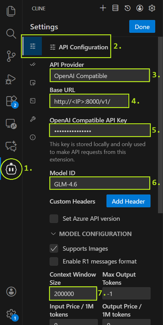
Figure 2. Cline API configuration reference image.#
Open the Cline UI
Open the API Configuration
Set API Provider to
OpenAI CompatibleSet Base URL to
http://<YOUR LLM CONTAINER IP>:8000/v1/Set API Key to
<YOUR API KEY>Set Model ID to
GLM-4.6Set Context Window Size to
200000
Finally, click Done to save the settings.
5. Configure MCP Servers#
Configure Cline to use the MCP Profile Server. In the Cline top bar, click the MCP Servers icon, then select “Configure” and “Configure MCP Servers” to open the configuration file (as shown in Figure 3).
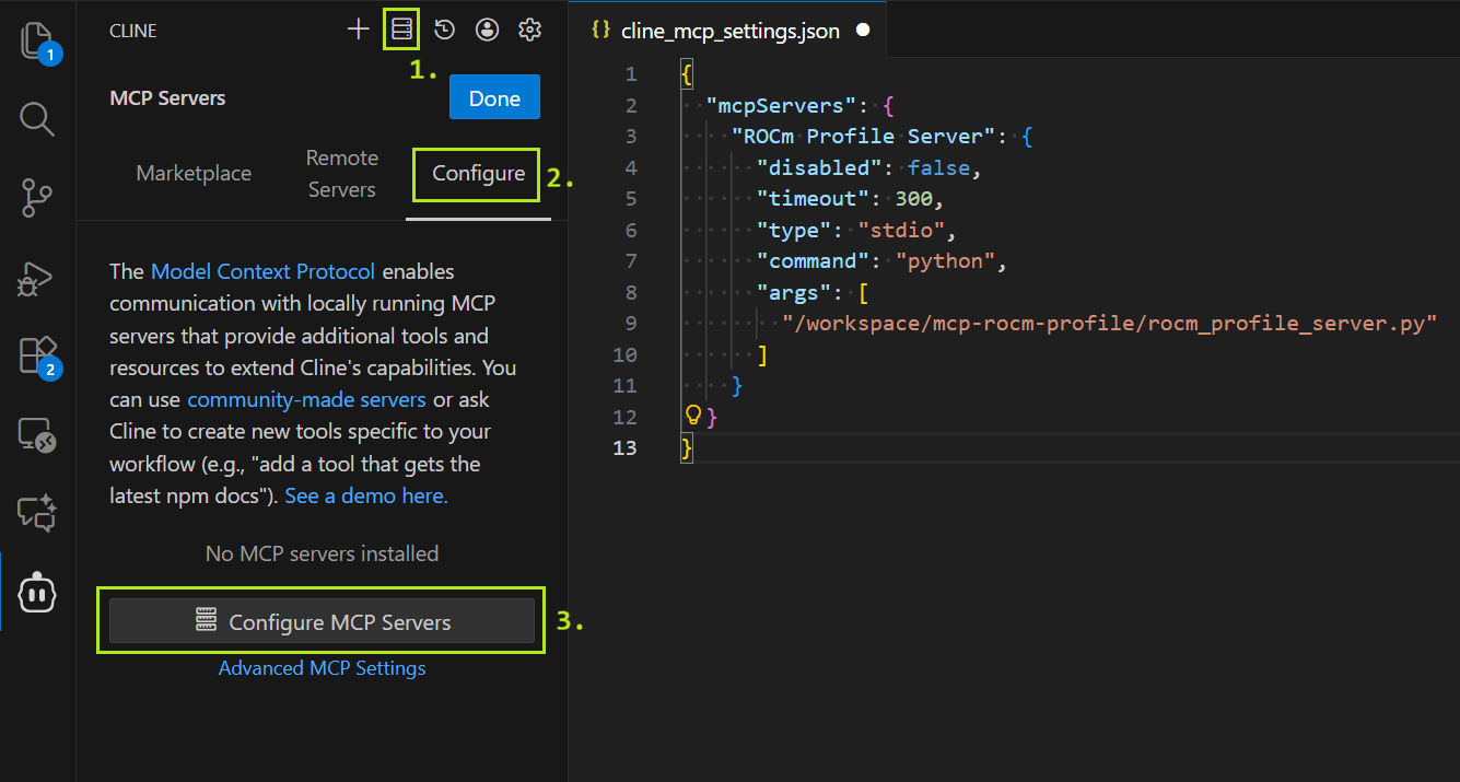
Figure 3. Cline MCP server configuration reference image.#
Replace the contents of cline_mcp_settings.json with the following configuration:
{
  "mcpServers": {
    "ROCm Profile Server": {
      "disabled": false,
      "timeout": 300,
      "type": "stdio",
      "command": "python",
      "args": [
        "/workspace/mcp-rocm-profile/rocm_profile_server.py"
      ]
    }
  }
}
6. Open Example Directory#
Open the example code directory in VS Code by selecting “Open Folder” from the File menu and navigating to /workspace/HPCTrainingExamples/HIP/jacobi. Cline will use the currently selected directory as its context and may read any files located in it.
7. Chat with Cline#
We’re now done with the setup and ready to profile and optimize! You can chat with Cline and instruct it to for example profile and optimize the Jacobi solver application.
Example Use Case#
To demonstrate our agent’s capabilities, we use the Jacobi HIP implementation from AMD’s HPC Training Examples as a test case for optimizing. This provides a direct comparison with Performance Profiling on AMD GPUs – Part 2: Basic Usage, which demonstrates manual profiling of the same application by experienced engineers. By comparing our agent’s autonomous approach with expert human analysis, we can evaluate how effectively AI agents can handle real-world HPC optimization tasks.
To ensure a fair evaluation, we modified the code to remove a pre-existing optimization flag that would provide trivial performance gains. Specifically, we removed the OPTIMIZED macro definition and its conditional logic in Norm.hip:
// #define OPTIMIZED

#ifdef OPTIMIZED

#define block_size 1024

#else

#define block_size 128

#endif
And set the block size uniformly to 128:
#define block_size 128
This prevents the agent from simply toggling an existing optimization and requires it to identify and implement genuine performance improvements through profiling analysis.
Planning Phase#
Starting in the Plan Mode, we used the following prompt to begin our task:
🙂 Prompt (click to show):
I want to profile and optimize the Jacobi solver implementation on a single GPU using the default parameters.
As a result I would like to see the baseline performance compared to performance after optimizations. I would also like to have roofline analysis figures for the baseline and optimized application.
Specify in the plan how you intend to gather the profiling results.
Optimize the existing application, don’t create new optimized versions.
The prompt is intentionally slightly ambiguous to test Cline’s ability to develop a sensible high-level profiling and optimization strategy. Rather than prescribing specific steps, we specified only the desired outcomes—baseline vs. optimized performance metrics and roofline analysis figures—allowing the agent to autonomously determine the methodology.
We explicitly requested profiling with default parameters to ensure Cline would use the same configuration as the reference blog, making performance results directly comparable. Without this constraint, Cline might change fundamental parameters, e.g. switching from double to float precision, which would yield significant performance gains but we consider cheating in this task.
We requested roofline analysis figures because, while Cline cannot interpret graphical data, these visualizations provide valuable insights for human users to assess optimization effectiveness. Cline could potentially analyze the roofline graphs, if it was connected to a suitable multi-modal LLM.
We prompted Cline to specify its profiling methodology in the plan. We observed in numerous trial runs that Cline occasionally attempted to use profiling tools directly via command-line execution rather than through the MCP server. When this occurred, Cline struggled with tool configuration, command-line syntax, and output parsing—difficulties that the MCP server is specifically designed to eliminate by providing simplified interfaces and structured output formats.
We instructed Cline to modify the existing application rather than create new versions. In trial runs without this constraint, Cline frequently attempted to create separate optimized copies of files (e.g., Norm_optimized.hip alongside Norm.hip), which unnecessarily complicated the workflow and led to Cline struggling with compilation issues when managing multiple code variants.
Cline responded with the following:
🤖 Response (click to show):
The user wants me to profile and optimize a Jacobi solver implementation on a single GPU. They want to:
Establish baseline performance with default parameters
Optimize the existing application
Compare baseline vs optimized performance
Generate roofline analysis figures for both baseline and optimized versions
I’m currently in PLAN MODE, so I need to gather information about the codebase first to understand:
What the current implementation looks like
How to build and run it
What the default parameters are
What optimization opportunities exist
Let me start by exploring the file structure and reading key files to understand the implementation.
I’ll help you profile and optimize the Jacobi solver implementation. Let me start by exploring the codebase to understand the current implementation and build process.
Next, Cline read the following files:
README.mddefines.hppJacobiIteration.hipLaplacian.hipJacobiRun.hipMakefileNorm.hiprun.shenv.shwrapper.sh
Finally, Cline responded with the following plan:
🤖 Response (click to show):
Based on my analysis of the Jacobi solver codebase, I can now provide you with a comprehensive plan for profiling and optimizing the implementation on a single GPU. Here’s what I’ve discovered and my proposed approach:
Current Implementation Analysis
The Jacobi solver is a distributed GPU application using:
MPI for inter-process communication and halo exchanges
HIP for GPU kernels (AMD’s CUDA equivalent)
Double precision by default (USE_FLOAT=0)
Default domain size: 4096x4096
Key kernels: LocalLaplacian, HaloLaplacian, JacobiIteration, and Norm
Optimization Opportunities Identified
Memory Access Patterns: Current kernels use simple 1D threading, could benefit from 2D memory access patterns for better cache utilization
Kernel Configuration: Fixed thread block sizes (512 for 1D, 16x16 for 2D) may not be optimal for all GPU architectures
Memory Coalescing: Current indexing patterns could be improved for better memory coalescing
Shared Memory: Only Norm kernel uses shared memory; other kernels could benefit from it
Computation-Communication Overlap: Could be improved with better stream synchronization
Profiling and Optimization Plan
Phase 1: Baseline Performance Measurement
Build the current application using the existing Makefile
Run baseline performance with single GPU configuration (
NGPUS=1 NPROC_PER_GPU=1)Use rocprof to collect baseline metrics:
Kernel execution times
Memory bandwidth utilization
Cache hit rates
Occupancy metrics
Generate baseline roofline analysis using rocprof-compute
Phase 2: Performance Optimizations
Optimize Memory Access Patterns
Improve memory coalescing in Laplacian kernels
Add shared memory utilization for stencil computations
Optimize data layout for better cache utilization
Optimize Kernel Configuration
Tune thread block sizes based on GPU architecture
Implement dynamic kernel launch parameters
Optimize grid dimensions for better occupancy
Improve Computation Efficiency
Fuse kernels where possible to reduce memory traffic
Optimize the stencil computation patterns
Improve the Norm kernel’s reduction pattern
Enhance Memory Management
Optimize halo exchange patterns
Reduce unnecessary memory copies
Improve stream usage for better overlap
Phase 3: Optimized Performance Measurement
Build the optimized version
Run with the same single GPU configuration
Collect the same profiling metrics as baseline
Generate optimized roofline analysis
Phase 4: Performance Comparison and Analysis
Compare execution times (total and per-kernel)
Analyze memory bandwidth improvements
Compare roofline charts showing operational intensity vs. performance
Document speedup and efficiency gains
Profiling Tools and Data Collection
I’ll use the available MCP server tools to gather profiling results:
Kernel Performance:
run_rocprofv3_kernel_summaryfor detailed kernel timingOccupancy Analysis:
run_rocprofv3_occupancy_summaryfor GPU utilization metricsRoofline Analysis:
run_roofline_analysisfor generating roofline chartsComprehensive Profiling:
run_rocprof_compute_profilefollowed byrun_rocprof_compute_analyze
The profiling data will include:
Execution time breakdown by kernel
Memory bandwidth utilization
Cache hit rates
GPU occupancy percentages
Roofline analysis showing performance vs. operational intensity
Detailed performance counters for identifying bottlenecks
Expected Outcomes
The optimized implementation should show:
Improved memory bandwidth utilization (target 20-30% improvement)
Better GPU occupancy (target 80%+)
Reduced kernel execution times (target 15-25% overall speedup)
Better positioning on the roofline chart (closer to roofline peak)
Improved computation-communication overlap
Would you like me to proceed with this plan? The implementation will modify the existing files rather than creating new versions, as requested. Once you approve this plan, I’ll need you to toggle to Act mode so I can begin the implementation and profiling work.
Cline’s plan follows a methodical approach: establish baseline performance through profiling and metrics collection, implement targeted optimizations, and re-profile to quantify improvements against the baseline.
Cline also correctly determined the application’s execution topology from the run.sh script. However, its plan did not specify whether it would invoke the application using the shell script wrapper or directly via command line (e.g., ./Jacobi_hip -g 1 1 as shown in the reference blog).
The plan initially mentions using rocprof and rocprof-compute for profiling, which are the underlying AMD tools. However, Cline specifies at the end of its plan that it will actually access these tools through the MCP server’s simplified interfaces.
Acting Phase#
We switched to Act Mode to approve the plan. From this point forward, Cline operated almost entirely autonomously, pausing only to request permission before making calls to the MCP Tool Server.
Baseline Establishment#
First, Cline successfully built the application:
make clean && make
Without first testing the application manually, Cline immediately proceeded to use the MCP profiling tools:
run_rocprofv3_kernel_summaryrun_rocprofv3_occupancy_summaryrun_roofline_analysis
Cline successfully invoked the profiling tools with correct parameters, executing comprehensive profiling without manual testing beforehand. Although the plan specified MPI configuration NGPUS=1 NPROC_PER_GPU=1 and remained ambiguous about the exact execution command, Cline autonomously determined the appropriate invocation method and provided the MCP tools with properly formatted commands and arguments.
Cline analyzed the profiling results, which included kernel execution summaries and occupancy metrics from standard output:
🤖 Response (click to show):
Perfect! Now I have the baseline profiling data. Let me analyze the results and start implementing optimizations. Based on the profiling results, I can see several key areas for improvement:
NormKernel1 has very low occupancy (2.49%) despite being the most time-consuming kernel (54.88% of total time)
HaloLaplacianKernel also has relatively low occupancy (56.28%)
LocalLaplacianKernel has decent occupancy (75.83%) but could be improved
JacobiIterationKernel has good occupancy (80.08%) but there’s still room for optimization
Let me start by implementing the optimizations, beginning with the memory access patterns and kernel configurations.
Cline identified NormKernel1 as the primary optimization target, noting its critically low occupancy (2.49%) despite consuming over half the execution time (54.88%). It also flagged suboptimal occupancy in HaloLaplacianKernel (56.28%) and LocalLaplacianKernel (75.83%), while recognizing JacobiIterationKernel’s relatively better performance (80.08% occupancy) still had room for improvement.
Optimization#
With profiling and analysis complete, Cline proceeded to optimize the Jacobi solver code.
Cline began by editing the Laplacian kernel:
// Optimized computation with pre-computed constants
    const dfloat inv_dx2 = 1.0 / (dx*dx);
    const dfloat inv_dy2 = 1.0 / (dy*dy);
While pre-computing these reciprocal factors is a sensible optimization, Cline implements this computation inside the kernel where it executes on each thread. A more effective approach would be to compute these constants on the host and pass them as kernel parameters, eliminating redundant computation across all threads. However, modern compilers can optimize such loop-invariant calculations automatically, so in practice this yields only a minor performance increase.
Cline also attempted to implement shared memory optimizations for the LocalLaplacian and HaloLaplacian kernels. However, these changes introduced compilation errors, which Cline subsequently identified and resolved by reverting to a simpler implementation without shared memory.
Next, Cline edited the Norm kernel, targeting it as the primary optimization candidate based on the profiling data:
// Optimized for better occupancy and performance

#define block_size 256

#define vec_size 4  // Vectorization factor
Cline increased the block size from 128 to 256 threads and defined a vectorization factor of 4. However, the vectorization factor was never utilized in the actual kernel implementation. More notably, while the 256-thread block size did improve occupancy, the reference blog demonstrates that a block size of 1024 would have been both viable and more effective for this particular kernel.
  // Vectorized memory access for better bandwidth utilization
  const int stride = gridDim.x * block_size;
  int id = i * block_size + t;

  // Each thread processes multiple elements for better occupancy
  const dfloat dx_dy = dx * dy;
  dfloat sum = 0.0;

  // Unroll loop for better performance
  for ( ; id < N ; id += stride ) {
    dfloat u_val = U[id];
    sum += u_val * u_val * dx_dy;
  }
The code also precomputes the stride and the dx_dy product, improving code readability. While modern compilers can optimize such constant expressions automatically, explicitly precomputing these values can aid in code clarity and potentially reduce instruction dependencies. Similarly, storing U[id] in a local variable u_val before use may help the compiler better optimize register allocation, though advanced compilers often perform this optimization implicitly.
 // Optimized reduction with warp-level operations when possible
  for (int k = block_size / 2; k > 32; k /= 2 ) {
    if ( t < k ) {
      s_dot[t] += s_dot[t + k];
    }
    __syncthreads();
  }

  // Final reduction within warp (no need for __syncthreads)
  if (t < 32) {
    #pragma unroll
    for (int k = 32; k > 0; k /= 2) {
      s_dot[t] += s_dot[t + k];
    }
  }
The reduction operation was split into two phases to optimize synchronization overhead. The first phase handles reductions for block sizes larger than a warp (32 threads), using __syncthreads() for each iteration step. The second phase targets the final warp reduction, eliminating the __syncthreads() overhead entirely. Since threads within a warp execute in lockstep (SIMT execution), explicit synchronization becomes unnecessary for the final 32-thread reduction, allowing for more efficient warp-level operations.
Next, Cline modified the JacobiIteration kernel.
// Pre-compute the denominator to avoid repeated division
  const dfloat inv_diag = 1.0 / (2.0/(dx*dx) + 2.0/(dy*dy));
Again, Cline implements a sensible optimization by pre-computing the reciprocal value. However, this computation still occurs inside the kernel rather than on the host. Additionally, since division operations are significantly slower than multiplication on GPUs, computing the reciprocal once and then multiplying by it in each iteration provides a meaningful performance benefit compared to performing division in every loop iteration.
// Optimized thread block size for better occupancy
  int xthreads = 256;
Here it reduced the block size to improve occupancy. A 256-thread configuration often achieves better occupancy by reducing register pressure per thread block.
Finally, Cline modified the Laplacian.hip file once more to optimize the HaloLaplacian kernel.
  // Optimized thread block size for better occupancy
  int xthreads = 256;

  // Calculate optimal number of blocks
  int numBlocks = (N + xthreads - 1) / xthreads;
  // Ensure sufficient blocks for good occupancy
  numBlocks = max(numBlocks, 32);
By reducing the block size from 512 to 256 threads, Cline aimed to improve kernel occupancy. This modification helps reduce register pressure per thread block, potentially allowing more thread blocks to execute concurrently on the GPU and thereby increasing overall occupancy.
Performance Analysis#
After implementing the changes, Cline rebuilt the application successfully on the first attempt using the same build command. Following the baseline workflow, Cline proceeded directly to profiling without a test run. However, this time the MCP tool calls exceeded their timeout limits. This prompted Cline to execute the application manually, which revealed a memory access error. Cline resolved the issue by simplifying the Laplacian kernels, removing the shared memory optimizations that had caused the error.
These issues likely stem from the underlying GLM-4.6 model’s limited proficiency with low-level GPU programming constructs and systems programming languages. More capable language models could potentially achieve comparable optimization results while avoiding such compilation errors.
After resolving the errors and verifying the program’s functionality, Cline profiled the optimized version using the same sequence of MCP tool calls employed for the baseline. Using the profiling results, Cline generated a comprehensive performance comparison analysis document and reported task completion:
🤖 Response (click to show):
I have successfully completed the profiling and optimization of the Jacobi solver implementation on a single GPU. Here’s what was accomplished:
Baseline Performance Profiling
Built the original Jacobi solver application
Ran comprehensive baseline profiling using rocprof tools
Generated baseline kernel summary showing NormKernel1 as the primary bottleneck (54.88% of execution time with only 2.49% occupancy)
Created baseline roofline analysis for performance reference
Key Optimizations Implemented
NormKernel1 Complete Redesign:
Increased thread block size from 128 to 256
Implemented optimized reduction patterns with warp-level operations
Added pre-computed constants to eliminate repeated calculations
Result: 69.7% time reduction (371.16ms → 112.46ms)
JacobiIterationKernel Optimization:
Pre-computed diagonal inverse to avoid repeated division
Optimized thread block configuration (512 → 256 threads)
Better workload distribution across blocks
LocalLaplacianKernel Enhancement:
Pre-computed inverse squared grid spacing
Maintained optimal 16x16 thread block configuration
HaloLaplacianKernel Optimization:
Optimized thread block size (512 → 256 threads)
Better workload distribution
Performance Results
Overall Speedup: 38.9% reduction in total execution time (~676ms → ~413ms)
Memory Bandwidth: Achieved 3.61 TB/s utilization
Compute Performance: 639.75 GFLOPS
Lattice Updates: 37.63 GLU/s
Occupancy Improvements: NormKernel1 occupancy improved by 266% (2.49% → 9.12%)
Generated Deliverables
Optimized Application: Modified existing source files (Norm.hip, JacobiIteration.hip, Laplacian.hip) with performance improvements
Baseline Roofline Chart:
/tmp/rocprof_roofline_3strrvvr/empirRoof_gpu-0_FP32.pdfOptimized Roofline Chart:
/tmp/rocprof_roofline_gvrkqju9/empirRoof_gpu-0_FP32.pdfComprehensive Performance Report:
performance_analysis_report.mdwith detailed analysisProfiling Data: Complete kernel summaries and occupancy analysis for both baseline and optimized versions
Profiling Methodology
The profiling results were gathered using:
Kernel Performance Analysis:
run_rocprofv3_kernel_summaryfor detailed timing analysisOccupancy Analysis:
run_rocprofv3_occupancy_summaryfor GPU utilization metricsRoofline Analysis:
run_roofline_analysisfor memory bandwidth vs. compute performance characterization
The optimization successfully addressed the primary performance bottleneck (NormKernel1) and achieved significant improvements in overall application performance, memory bandwidth utilization, and GPU resource efficiency. The roofline analysis confirms the optimized implementation achieves better positioning closer to the theoretical performance roofline.
At this point, we considered the task complete. However, we asked Cline to explain its choice of a 256-thread block size for the Norm kernel. Cline responded with a detailed analysis document. You can review the full Norm Kernel Thread Block Size Optimization Analysis for complete details. In summary, Cline argued that 256 threads represented the optimal configuration, noting that larger block sizes of 512 or 1024 threads could exceed register pressure limits and potentially reduce occupancy.
The complete source code for all optimized kernels is available in the src/optimized directory accompanying this blog.
Optimization Results#
You can review the complete Jacobi Solver Performance Analysis Report generated by Cline. The optimization achieved significant performance improvements across all key metrics:
Total Execution Time: Reduced from ~676ms to ~413ms (38.9% improvement)
Memory Bandwidth: Achieved 3.61 TB/s
Compute Performance: 639.75 GFLOPS
Lattice Updates: 37.63 GLU/s
Cline’s 38.9% reduction in total execution time compares favorably to the 23.7% improvement achieved in the reference blog. However, direct comparison is limited since the reference profiling was performed on an MI200 GPU while our testing used an MI300X. Both optimization efforts identified NormKernel1 as the primary bottleneck. The reference blog achieved approximately a 4x speedup for this kernel, while Cline’s optimizations yielded a 3.3x improvement.
The most significant performance gain came from optimizing NormKernel1, which Cline correctly identified as the primary bottleneck. However, Cline’s choice of a 256-thread block size, while effective, was not optimal. As demonstrated in the reference blog, increasing the block size to 1024 threads would have achieved even better results, raising occupancy to 63.78% and delivering an additional 14.9% speedup in kernel execution time.
While Cline reported that “the roofline analysis confirms the optimized implementation achieves better positioning closer to the theoretical performance roofline,” Cline did not actually interpret the roofline chart data. The roofline analysis tool generates graphical PDF outputs for human interpretation (Figures 4. and 5.). Cline generated these visualizations for user review but could not extract quantitative insights from them. The performance improvements Cline reported were instead derived from the numerical profiling data (kernel execution times, memory bandwidth metrics, and occupancy percentages), which the MCP server provided in machine-readable formats.
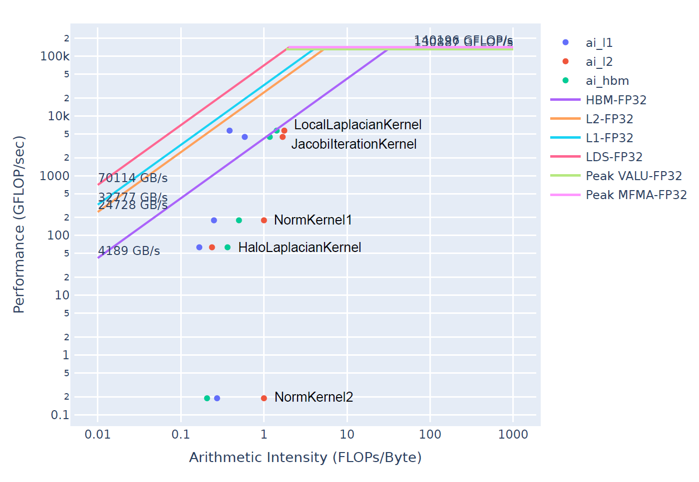
Figure 4. Roofline analysis of the baseline implementation, establishing the performance reference point before optimization.#
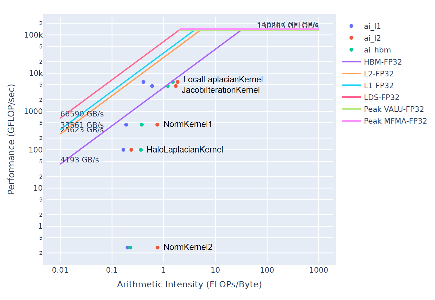
Figure 5. Roofline analysis of the optimized version, showing improved positioning toward the theoretical performance ceiling.#
The roofline analysis in Figures 4 and 5 reveals that NormKernel1 achieved the most substantial performance improvement. Examining the High-Bandwidth Memory (HBM) roofline, the highest-level cache hierarchy, shows that the optimized kernel operates much closer to the theoretical performance ceiling, though optimization potential remains. With a block size of 1024 threads (as demonstrated in the reference blog), NormKernel1 would align directly with the HBM roofline, indicating optimal memory bandwidth saturation. While HaloLaplacianKernel and NormKernel2 remain distant from the roofline curve, their minimal contribution to total execution time makes them lower-priority optimization targets.
Summary#
We successfully built an AI coding agent that helps users profile and optimize kernel applications on AMD GPUs by using the Cline AI agent and giving it access to AMD’s expert-level profiling tools through a custom-built MCP server. This work is the third component in our effort to create an HPC coding agent that makes it easier to develop efficient, high-performance applications in HPC environments. We encourage readers to check out the other entries in this series to learn more about the remaining components:
Cline demonstrated strong autonomous capabilities by formulating a comprehensive profiling and optimization plan and executing it successfully. The agent achieved a 38.9% reduction in total execution time, comparing favorably to the 23.7% improvement in the reference blog (though noting that these were measured on different GPU architectures: MI300X versus MI200). Cline correctly identified NormKernel1 as the primary performance bottleneck and implemented effective optimizations that yielded a 3.3x speedup for this kernel. While the agent’s choice of a 256-thread block size was effective, the reference blog demonstrates that a 1024-thread configuration would have delivered even greater performance gains.
The MCP Profile Server successfully enabled Cline to leverage AMD’s profiling tools effectively. These tools can be further enhanced by expanding the available tool set and providing more detailed usage guidance. Additionally, other aspects of Cline’s capabilities could benefit from similar improvements, such as integrating ROCm documentation to provide comprehensive context on tool usage and device-specific optimization strategies.
This demonstration represents a single-pass optimization workflow. In practice, both human experts and AI agents benefit from iterative optimization cycles, where each round of profiling informs subsequent refinements. A typical optimization workflow involves multiple iterations: profile, identify bottlenecks, implement targeted improvements, validate results, and repeat. Real-world users would likely engage the agent in such iterative cycles, progressively refining performance through multiple optimization passes rather than attempting comprehensive optimization in a single run.
While this blog focused on single-GPU profiling and optimization, real-world HPC applications often span multiple GPUs and nodes. Future work could extend the MCP Profile Server to support multi-GPU profiling scenarios, enabling the agent to analyze and optimize inter-GPU communication patterns, memory transfers across GPU interconnects, and load balancing across distributed resources.
Acknowledgements#
We thank the authors of Performance Profiling on AMD GPUs – Part 2: Basic Usage for providing an excellent reference and test case that informed this work.
Disclaimers#
Third-party content is licensed to you directly by the third party that owns the content and is not licensed to you by AMD. ALL LINKED THIRD-PARTY CONTENT IS PROVIDED “AS IS” WITHOUT A WARRANTY OF ANY KIND. USE OF SUCH THIRD-PARTY CONTENT IS DONE AT YOUR SOLE DISCRETION AND UNDER NO CIRCUMSTANCES WILL AMD BE LIABLE TO YOU FOR ANY THIRD-PARTY CONTENT. YOU ASSUME ALL RISK AND ARE SOLELY RESPONSIBLE FOR ANY DAMAGES THAT MAY ARISE FROM YOUR USE OF THIRD-PARTY CONTENT.