Large language model inference optimizations on AMD GPUs#

15, Mar 2024 by .
Large language models (LLMs) have transformed natural language processing and comprehension, facilitating a multitude of AI applications in diverse fields. LLMs have various promising use cases, including AI assistants, chatbots, programming, gaming, learning, searching, and recommendation systems. These applications leverage the capabilities of LLMs to provide personalized and interactive experiences, which enhances user engagement.
LLMs use transformer architecture to solve gradient vanishing and explosion problems. This architecture allows for easy parallelization of self-attention, making it possible to efficiently utilize multiple GPUs. Other architectures, such as recurrent neural networks (RNN) and its variants (e.g., LSTM and GRU), struggle when handling long sequences of words.
Despite impressive capabilities, LLMs like GPT and Llama require aggressive optimization before being deployed for commercial applications due to their large parameter size and autoregressive sequential processing behavior. Many efforts have been made to improve the throughput, latency, and memory footprint of LLMs by utilizing GPU computing capacity (TFLOPs) and memory bandwidth (GB/s).
We’ll discuss these optimization techniques by comparing the performance metrics of the Llama-2-7B and Llama-2-70B models on AMD’s MI250 and MI210 GPUs.
Model characteristics: Llama2-7b and Llama2-70b#
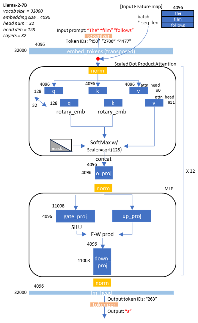
The Llama2-7b and 70b models are capable of handling 32,000 vocabulary words. These models can process a maximum length of 4,096 token sequences. Llama2 optimized its training and inference performance by adopting the following new features:
Sigmoid Linear Unit (SiLU) activation: Replaces the commonly used Rectified Linear Unit (ReLU) to reduce the vanishing gradient problem for smoother activation.
Rotary positional embedding: Reduces the computing costs of a classic absolution positional embedding layer, while retaining the positional information of the token sequence.
Pre-normalization: The LlamaRMSNorm module normalizes the input instead of the output, which reduces the gradient vanishing and explosion problem.
In the Llama-2-7b model, there are 32 attention heads in the self-attention module; each head has 128
dimensions. The Multilayer Perceptron (MLP) module has 11,008 intermediate size and it is composed
of three layers: gate_proj, up_proj, and down_proj.

Based on their behaviors, LLMs are categorized into the following:
Masked Language Model (MLM): Predicts a new masked word between the provided context words. BERT is an example of an MLM.
Causal Language Model (CLM): Predicts the next word after the provided context words. One well-known CLM example is GPT text generation. CLM is also known as an autoregressive token generation model due to its sequential processing behavior.
In this blog, we focus more on Llama2 CLM.

The token generation in a CLM is performed in the following two phases:
Time to first token (TTFT): The time taken to generate the first token. Prefill latency is defined as the average TTFT across requests. In the following figure, TTFT is the time taken to generate “in” from the input prompt to “The largest continent”.
Time per output token (TPOT): The time taken to generate each output token in an autoregressive manner. Output decoding latency is defined as the average TPOT across requests, and is usually estimated using the time taken during the output decoding phase. In the following figure, TPOT is the decoding latency of “the”.
The TTFT and TPOT are used to calculate the latency in a CLM:
latency = TTFT + TPOT * (max_new_tokens - 1)
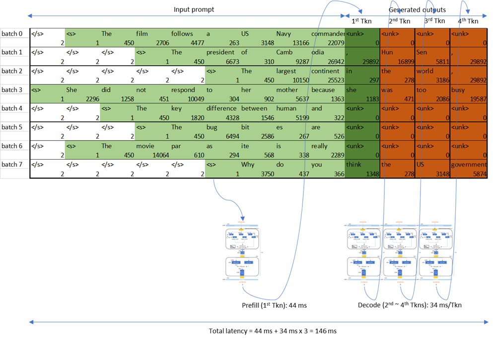
The dimension of the input in the prefill phase after token embedding is proportional to batch_size * input sequence_length. The tokens in the prefill phase are processed at the same time. However, the input to the output decoding, after token embedding, is proportional to batch_size; tokens in this phase are processed sequentially. This is why the output decoding operation is composed of tall and skinny GEMM (or GEMV) when the batch size is 1.
For the sake of simplicity, we use greedy-decoding for generated tokens, which is known to have minimal token decoding overhead from output logits. In real chatbot scenarios where rich and unexpected output token generation is allowed, it’s better to consider sampling-based decoding and higher beam width. But, in the greedy-decoding scheme, the autoregressive CLM generates top-1 tokens from the model output logit.
Device characteristics: MI210#
AMD’s Instinct ™ MI210 has a maximum computing capacity of 181 TFLOPs at the FP16 datatype. To fully leverage matrix core performance, the matrix dimension of GEMM should be large enough. The LLM prefill decoding phase with large batch uses large input matrices and can benefit from the high performance of matrix cores. With MI210, during the prefill phase where the prompt sequence length and batch size are large, the GEMM operations are compute-bound.
MI210 can provide a maximum double data rate (DDR) memory bandwidth up to 1.6 TB/s. The output decoding processes tokens sequentially. This autoregressive decoding has only one dimension of sequence length (which makes the tall and skinny GEMM or GEMV) where the operations are memory-bound. Due to this sequential nature of LLM output token generation, the output decoding benefits from DDR bandwidth.
MI250 is composed of two Graphics Compute Dies (GCD) from MI210. Therefore, MI250 has two times the computing capacity, memory size, and memory bandwidth of MI210. The LLM can be assigned to the two silicon dies of MI250 in tensor parallel (TP), pipeline parallel (PP), or data parallel (DP) styles of model parallelism. This data parallel can double the LLM throughput with a two-fold model parameter duplication overhead. The lack of overhead causes the tensor parallel to be widely used due to its ability to fit larger LLM onto high-capacity MI250 DDR with some collective operation synchronization overheads.
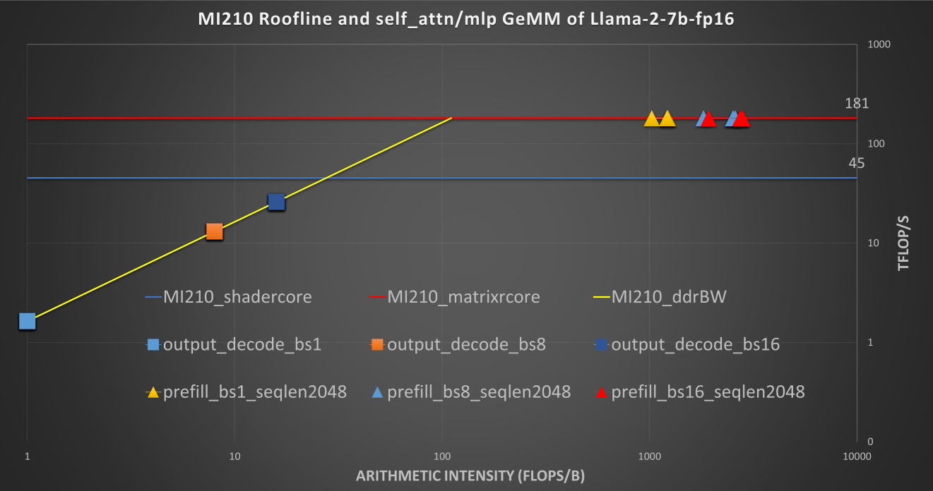
In the preceding figure, note that the roofline of the MI250 single GCD is similar to that of MI210.
Software setup#
Installing ROCm on the host#
To install ROCm 6.0 on the host, see the install instructions.
Setting up docker#
To set up the official PyTorch ROCm Docker container, use the following command:
docker run -it --network=host --device=/dev/kfd --device=/dev/dri --group-add=video --ipc=host --cap-add=SYS_PTRACE --security-opt seccomp=unconfined --shm-size 8G --name llm_optimization rocm/pytorch:rocm6.0_ubuntu22.04_py3.9_pytorch_2.0.1
Configuring the library and toolkit#
Run the following command to install PyTorch 2.3 nightly:
pip3 uninstall torch torchvision torchaudio pytorch-triton-rocm -y
pip3 install --pre torch torchvision torchaudio --index-url https://download.pytorch.org/whl/nightly/rocm6.0
For library setup, refer to Hugging Face’s transformers.
For toolkit setup, refer to Text Generation Inference (TGI).
Optimization comparison of Llama-2-7b on MI210#
Prefill latency

Output decoding latency

Default machine-learning framework#
PyTorch 2 supports two running modes: eager and compilation. Eager mode is the default PyTorch mode, in which the operators of a model are run sequentially as soon as they are encountered during runtime. Compilation mode is covered under the LLM inference optimization techniques.
To run a LLM decoder model (e.g., Llama-2), Hugging Face provides the transformers library to run models on top of PyTorch.
The transformers library uses various token generation options as arguments in its APIs. In this blog, to fairly compare the performance of each optimization, these options are deployed:
Prefill: With a 2,048 sequence length prompt, the prefill latency increases according to the batch size, because large GEMM computation during the prefill is compute-bound.
Output decoding: The output decoding latency doesn’t increase much when the batch size increases, as the arithmetic intensity of GEMM during this phase is still memory bandwidth-bound.
LLM inference optimization techniques#
Here, we discuss the various LLM inference optimization techniques.
PyTorch compilation mode#
In PyTorch compilation mode, a model is synthesized into a graph and then lowered to prime operators. These operators are compiled using TorchInductor, which uses OpenAI’s Triton as a building block for GPU acceleration. One advantage of PyTorch compilation mode is that its GPU kernels are written in Python, making it easier to modify and extend them. PyTorch compilation mode often delivers higher performance, as model operations are fused before runtime, which allows for easy deployment of high-performance kernels.
To run an LLM decoder model (e.g., Llama2) in PyTorch compilation mode, specific layers of the model
must be explicitly assigned as compilation targets. The PyTorch compilation mode requires
recompilation with dynamic input shapes of the LLM decoder model, where the input batch size and
sequence length can change during runtime. To support recompilation with dynamic input shapes, set
the parameter dynamic=True.
for i in range(model.config.num_hidden_layers):
    model.model.decoder.layers[i].self_attn = torch.compile(model.model.decoder.layers[i].self_attn, backend="inductor", mode="default", dynamic=True)
Prefill: The prefill latency is significantly reduced. But, for LLM decoder models, it still suffers huge initial recompilation overhead for various batch sizes and input sequence lengths. The prefill latency is measured after the initial recompilation (warmups).
Output decoding: The output decoding latency is slightly better, because the model was partially compiled. However, the graph fell back to eager mode due to the dynamic shapes of partial key/value caches. There’s an effort to address this issue (known as static key/value cache). The static key/value cache, along with
torch.compile, shows much better output decoding performance, but we don’t cover this in our blog.
Flash Attention v2#
The Flash Attention (flash_attention) algorithm is designed to
address the large memory movements required for the query, key, and value components of the
Multi-head Attention (MHA) module in a transformer. This is
achieved by tiling the partial queries and storing them in a faster cache memory, rather than constantly
reading from the slower external DDR memory during MHA computations.
flash_attention v2](https://arxiv.org/abs/2307.08691) maximizes parallelism over long input sequence
lengths, leading to a significant performance boost over the native MHA.
You can seamlessly use the
flash_attention v2 module for ROCm with the latest
transformers library from Hugging Face.
from transformers import AutoModelForCausalLM, AutoTokenizer
model = AutoModelForCausalLM.from_pretrained(model_id, attn_implementation="flash_attention_2")
Prefill: The Flash Attention modules significantly reduce the prefill processing latency for large batch sizes and long sequence lengths, as MHA matrix dimensions are proportional to these. This leads to more gains for the flash attentions.
Output decoding:
flash_attentionisn’t effective during the output decoding phase, as the sequence length is just 1.
Memory-efficient multi-head-attention#
Memory-efficient, multi-head-attention (Xformers) is a collection of customizable modules from Meta.
They’re used to optimize transformers. The key feature of Xformers is the memory-efficient MHA
module that can significantly reduce memory traffic during MHA processing. This module uses a
similar algorithm to flash_attention to reduce the DDR read or write bandwidth.
You can seamlessly integrate Xformers’ memory-efficient MHA module for ROCM into Hugging Face’s transformers library.
Prefill: Memory-efficient MHA also significantly reduces the prefill processing latency for large batch sizes and long sequence lengths, for the same reason as
flash_attention v2.Output decoding: Xformers isn’t effective during the output decoding phase, as the sequence length is just 1.
Paged attention (vLLM)#
Paged attention (paged_attention) from the vLLM inference
system is an algorithm that can efficiently reduce the memory consumption, and decrease the latency
by two to four times during the output decoding phase. Paged attention manages Key and Value
cache (K-V cache) during the output decoding phase by using virtual memory and paging to reduce
memory fragmentation. Conventional K-V caching pre-allocates memory for maximum output token
lengths (2,048 or 4,096, depending on the model), which can cause memory fragmentation if the
actual decoding length is shorter. This algorithm’s virtual memory with paging can save K-V cache
memory when beam search is large and multiple requests are run in parallel.
vLLM's paged_attention module for ROCm is currently available.
Prefill: Paged attention isn’t effective during the prefill. as this phase doesn’t utilize K-V cache.
Output decoding: Paged attention can significantly reduce the decoding latencies.
PyTorch TunableOp#
PyTorch TunableOp allows you to use high-performance rocblas and hipblaslt libraries for GEMM. It profiles the LLM and prepares the best-performing GEMM kernels for each MHA and MLP modules. During runtime, the best-performing GEMM kernels are launched instead of PyTorch built in the GEMM kernels.
PyTorch TunableOp is available now.
Prefill: Combined with
flash_attention v2, PyTorch TunableOp shows significant performance increases in different batch sizes.Output decoding: With paged attention, PyTorch TunableOp also significantly reduces the latency for tall and skinny GEMM (or GEMV). Therefore, output decoding performance benefits the most from rocBLAS and hipBLASLt GEMMs.
Multi-GPU LLM inference optimization#
Prefill latency
Output decoding latency

Hugging Face Text Generation Inference#
Scaling out multi-GPU inference and training requires model parallelism techniques, such as TP, PP, or DP. TP is widely used, as it doesn’t cause pipeline bubbles; DP gives high throughput, but requires a duplicate copy of parameters loaded to GPU DDRs.
In this blog, we use TP to split the model across multiple GPUs and Hugging face’s
TGI to measure multi-GPU LLM inference.
Hugging Face’s TGI implementation of ROCm-enabled flash_attention and paged_attention,
compatibility with PyTorch TunableOp, and scope for ROCm-enabled quantizations (such as GPTQ)
makes it a good choice.
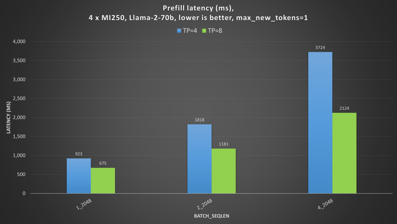
One server with 4 x MI250 has a total of 8 graphics compute dies (GCDs). Each GCD has 64 GB of HBM.


To fully utilize multiple MI250 GPUs, you need to consider the interconnect bandwidth between the GPU’s GCDs, as the inter-GCD connections have non-uniform throughput. For example, with TP=4, using GCD#0,1,4,6 together gives the best performance, as the collective operations (such as all-reduce or all-gather) cause less synchronization overhead in TP.
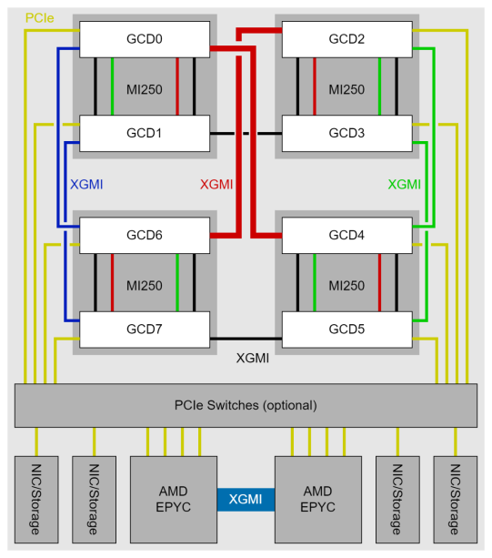

With non-uniform memory access (NUMA) balancing enabled, the GPU must wait for the preemptive memory management unit (MMU) notifier changes derived from page faults. Therefore, disabling NUMA balancing is recommended in order to keep the periodic automatic balancing from interfering with GPU operations.
echo 0 > /proc/sys/kernel/numa_balancing
Prefill and output decoding: the TP=8 (8 GCDs) case shows better prefill and output decoding latencies than TP=4 (4 GCDs). The latency enhancement is not doubled, as collective operations to synchronize MHA and MLP for every layer is also a huge latency bottleneck.
Summary#
In this blog, we introduced several software optimization techniques to deploy state-of-the-art LLMs
on AMD CDNA2 GPUs. These include PyTorch 2 compilation, Flash Attention v2, paged_attention,
PyTorch TunableOp, and multi-GPU inference. These have all been well-adopted by the AI community.
Using these optimizations, you can enjoy up to three times the out-of-the-box acceleration, depending
on batch size and input sequence length.