Utilizing AMD Instinct GPU Accelerators for Weather and Precipitation Forecasting with NeuralGCM

Utilizing AMD Instinct GPU Accelerators for Weather and Precipitation Forecasting with NeuralGCM#

March 19, 2026 by Nhat Vo.

8 min read. | 1887 total words.

Applications & models

AI

In recent years, the landscape of weather forecasting has evolved tremendously, employing cutting-edge AI technologies to enhance prediction accuracy and speed. In previous blogs, we have demonstrated how to run several state-of-the-art AI weather forecasting models, such as Pangu-Weather, GenCast, and Aurora. Following that, this blog focuses on emerging trends in weather forecasting models, particularly the innovative NeuralGCM, which melds the strengths of General Circulation Models (GCMs) and Machine Learning (ML). We will briefly outline the design of NeuralGCM and its hybrid approach for weather and precipitation forecasting. We will then go through the required environments, installation steps, and the inference process for generating forecasts and creating plots to compare the outputs to the ground truth provided by ERA5 data.

Traditional Methods and Machine Learning Innovations#

GCMs#

GCMs [1] are complex mathematical frameworks that represent the physical processes of the atmosphere, oceans, and land surface. Using GCMs to solve the dynamics of the Earth’s atmosphere is the basis of weather and climate prediction. By dividing the Earth into a three dimensional grid, GCMs use equations of fluid dynamics and thermodynamics, to simulate how the planetary atmosphere and ocean move across the globe.

The primary drawback of traditional GCMs is that they rely on human designed, simplified rules of thumb, i.e., parameterizations, to represent unresolved physical processes that occur at scales smaller than the model’s grid such as clouds, radiation and precipitation. Because these manual processes are computationally expensive yet physically incomplete, they create a computational bottleneck that forces a tradeoff between forecasting accuracy and processing speed. Furthermore, since these separate modules are often developed independently, they can interact inconsistently, leading to structural errors and model drift that degrade long-term prediction reliability.

ML-based weather forecasting#

ML techniques offer an alternative to traditional GCMs, replacing intricate mathematical processes with advanced ML models. By training on the reanalysis ERA5 dataset [2], recent ML-based weather prediction systems have successfully delivered cutting-edge deterministic forecasts for 1 to 10 days weather predictions, achieving significantly faster inference speeds [3], [4].

ML approaches still contain some notable limitations. They have not yet outperformed existing GCMs in long-term forecasts, often producing overly smooth and unrealistic results when optimized for extended periods. This issue arises because most ML models are trained to minimize error. If a model predicts an incorrect outcome, it incurs a large error as a penalty. As forecasts extend further into the future, the trained model tries to minimize the error by generating the average of all possible predictions, resulting in smooth predictions.

Additionally, ML approaches commonly emphasize deterministic forecasts, overlooking crucial calibrated uncertainty estimates. This is because they are usually trained to provide one specific answer for every prediction and tend to overlook uncertainty, which is an important factor in weather forecasting. Recently, some attempts have been made to produce probabilistic forecasts similar to the ensemble forecasting systems of physics-based weather models. Among the possible approaches, diffusion models are capable of sharpening atmospheric features in forecasts due to their random behavior. A significant development in the field is GenCast [9], which applies generative diffusion techniques to create detailed, ensemble-based weather predictions with high spatial resolution.

NeuralGCM#

Hybrid models integrate GCMs with ML to replace the conventional physical parameterizations in GCMs with ML-driven approaches. The idea of a hybrid approach is to combine the mathematical certainty of physics with the raw speed of machine learning that handles complex, small scale calculations. However, the AI modules in previous hybrid models were often trained individually and were not integrated or trained jointly with the physics-based weather modules, which often led to drifting results and crashes. In contrast, recent modern frameworks like NeuralGCM [5], [6] are designed to be fully integrated and differentiable. This allows the AI to learn while interacting with the laws of physics in realtime, resulting in a more stable, accurate, and physically consistent forecast. NeuralGCM delivers physically grounded forecasts with accuracy comparable to the world’s leading models. It offers high performance across diverse timelines from short term 15 days weather outlooks to long range climate projections spanning entire decades.

Overview of NeuralGCM#

Learned Encoder and Decoder#

The Learned Encoder and Decoder serve as the interface between raw ERA5 observational data on pressure coordinates and the model state in sigma coordinates. Seven atmospheric variables are considered: geopotential, u/v component of wind, temperature, specific cloud water, specific cloud ice, and specific humidity. To convert ERA5 data from fixed pressure levels to the sigma levels (terrain following coordinates), the Encoder performs vertical interpolation. This is achieved by calculating the pressure at each level using \(\sigma = p/p_{s}\), where \(p_{s}\) is the surface pressure. More discussions of the sigma coordinate can be found in our previous blog post. For each relevant atmospheric variable, the model uses log-linear interpolation to ensure smooth transitions between these vertical layers. The Decoder reverses this operation by mapping model state on sigma coordinates back to ERA5 snapshot on pressure coordinates. The Encoder and Decoder also incorporate a correction, calculated using a learned neural network with the same architecture as the learned physics module, into the interpolation results. The correction helps reduce the initialization shock that arises when mapping the ERA5 data to the model’s grid. The initialization shock refers to the occurrence of unwanted high frequency gravity waves in weather forecasting models, primarily caused by imbalances between the initial observed wind and mass fields, as well as discrepancies between the model and the actual atmosphere [8]. This shock can trigger artificial, high frequency oscillations that have the potential to contaminate the forecasts.

Dynamical Core#

The Dynamical Core is a physics engine that solves the Primitive Equations, which are a simplified version of the Navier-Stokes equations for a rotating sphere under hydrostatic balance. These equations govern the conservation of momentum, mass, and energy, expressed through variables like horizontal wind, temperature, and surface pressure. This module uses a spectral transform method to solve these equations, converting spatial data into spherical harmonics to compute horizontal derivatives with high precision. The primary input variables are the encoded global atmospheric state of the Encoder module. The output is the dynamic tendency, which represents the calculated rates of change for atmospheric state variables such as vorticity, divergence, and temperature, due to large scale atmospheric motion. Because the core is written in a differentiable framework (JAX), it can provide gradients for the neural network training process. This allows the ML components to learn how to fill the gaps caused by unresolved physics. By solving the big picture fluid dynamics mathematically, it provides a stable backbone that prevents the unphysical drift common in pure ML models.

Learned Physics Module#

The Learned Physics Module replaces traditional, hand coded parameterizations with a deep neural network, typically a Multi Layer Perceptron (MLP) with residual connections. This module takes the current atmospheric state \(x_{t}\), along with its spatial derivatives and auxiliary forcings like solar radiation and land-sea masks, as its input. Similar to the dynamic tendency, the output of this module is the physics tendency \(x_{\text{phys}}\), which accounts for the seven atmospheric variables in ERA5. To produce the total change in the atmosphere, the model combines these outputs with the Dynamical Core’s outputs \(x_{dym}\) through simple addition: \(x_{total} = x_{dym} + x_{phys}\). This additive structure allows the AI to act as a correction term to the deterministic fluid dynamics. The module is trained online over multiple time steps, meaning it learns to maintain stability over long rollout periods and avoids the inconsistencies often found when separate hand coded schemes interact. Finally, the ODE solver takes the combined tendencies from the dynamical core and the learned physics module to compute the state at the next time step using semi-implicit ODE solvers by partitioning dynamical tendencies into implicit and explicit terms.

Learned Precipitation#

Learned precipitation is an additional neural network for predicting precipitation (\(P\)) and evaporation (\(E\)). The precipitation network is like the Learned Physics Module network, but it is much smaller and the inputs are slightly different. Compared to the Learned Physics, the Learned Precipitation network does not take the spatial derivative of atmospheric states as the input. During training, the model is initialized with ERA5 variables but is specifically optimized to match the high resolution Global Precipitation Measurement (IMERG) satellite dataset [7]. The evaporation is also diagnosed by enforcing water budget in the column.

\[P - E = \frac{1}{g} \int_{0}^{1} \sum_{i} \left( \frac{dq}{dt} \right)_{i}^{NN_{\text{tend}}} p_{s} d\sigma \qquad (1)\]

where \(p_{s}\) is the surface pressure, and the inner summation is the sum of the water species tendencies predicted by the Learned Physics neural network.

Prerequisites#

Docker®: See Install Docker Engine for installation instructions.

ROCm kernel-mode driver: As described in Running ROCm Docker Containers you need to install amdgpu-dkms.

MI300X (or other compatible GPU): See System requirements (Linux) for more details.

AMD Container Toolkit: See Quick Start Guide for installation and corresponding ROCm blog.

Installation and setup#

To use NeuralGCM on AMD Instinct GPUs, we can use one of the ROCm Docker images:

rocm/dev-ubuntu-22.04:7.0.2-complete

The docker image can be downloaded simply by invoking the following:

docker pull rocm/dev-ubuntu-22.04:7.0.2-complete

We can launch a container running the image with the following command together with AMD Container Toolkit

docker run -d \
    --runtime=amd \
    -e AMD_VISIBLE_DEVICES=all \
    --name neuralgcm \
    -v $(pwd):/workspace/ \
    rocm/dev-ubuntu-22.04:7.0.2-complete \
    tail -f /dev/null

If you do not have the AMD Container Toolkit installed, you can run the following command instead:

docker run -d \
    --device=/dev/kfd \
    --device=/dev/dri \
    --group-add video \
    --name neuralgcm \
    -v $(pwd):/workspace/ \
    rocm/dev-ubuntu-22.04:7.0.2-complete \
    tail -f /dev/null

When the container is running, you can now open a new interactive shell in the container by running the following:

docker exec -it neuralgcm /bin/bash

In the new session, move to the workspace directory and install the NeuralGCM libraries and required dependencies:

cd /workspace
python3 -m pip install https://github.com/ROCm/rocm-jax/releases/download/rocm-jax-v0.6.0/jaxlib-0.6.0-cp310-cp310-manylinux2014_x86_64.whl
python3 -m pip install jax==0.6.0 jax-rocm7-pjrt jax-rocm7-plugin
apt update
apt install libdw1
python3 -m pip install neuralgcm gcsfs
python3 -m pip install matplotlib

We can verify the JAX on ROCm installation

python3 -c 'import jax, numpy as np; print("=" * 60); print("JAX Configuration:"); print("Available devices:", jax.devices()); print("Default device:", jax.devices()[0]); print("JAX version:", jax.__version__); print("NumPy version:", np.__version__); print("=" * 60)'

If JAX is configured properly on AMD Instinct hardware, you should see output similar to the following:

============================================================
JAX Configuration:
Available devices: [RocmDevice(id=0)]
Default device: rocm:0
JAX version: 0.6.0
NumPy version: 2.2.6
============================================================

We are now ready to run NeuralGCM inference on the AMD Instinct hardware!

Running inference#

First of all, we need to import the necessary Python packages. The bare minimum required can be imported with:

import os
import gcsfs
import jax
import numpy as np
import pickle
import xarray
import matplotlib.pyplot as plt
from dinosaur import horizontal_interpolation
from dinosaur import spherical_harmonic
from dinosaur import xarray_utils
import neuralgcm

The next step is to create and load the model checkpoint. NeuralGCM provided 6 checkpoints, 4 for weather and climate forecast, and 2 for precipitation weather forecast. All of them can be found at pre-trained model checkpoints - NeuralGCM documentation. We can select the model we want to load. In this case we select the 0.7° deterministic checkpoint:

# Load a pre-trained NeuralGCM model
model_name = 'v1/deterministic_0_7_deg.pkl'  #@param ['v1/deterministic_0_7_deg.pkl', 'v1/deterministic_1_4_deg.pkl', 'v1/deterministic_2_8_deg.pkl', 'v1/stochastic_1_4_deg.pkl', 'v1_precip/stochastic_precip_2_8_deg.pkl', 'v1_precip/stochastic_evap_2_8_deg.pkl'] {type: "string"}

gcs = gcsfs.GCSFileSystem(token='anon')
with gcs.open(f'gs://neuralgcm/models/{model_name}', 'rb') as f:
  ckpt = pickle.load(f)

model = neuralgcm.PressureLevelModel.from_checkpoint(ckpt)

Next, we will load the ERA5 data from GCP/Zarr and select the start and end times for the weather forecasting. We also slice the ERA5 data at 24-hour intervals:

# Load ERA5 data from GCP/Zarr
print("Loading ERA5 data from GCP/Zarr...")
era5_path = 'gs://gcp-public-data-arco-era5/ar/full_37-1h-0p25deg-chunk-1.zarr-v3'
full_era5 = xarray.open_zarr(
    era5_path, chunks=None, storage_options=dict(token='anon')
)

demo_start_time = '2020-03-18'
demo_end_time = '2020-03-22'
data_inner_steps = 24  # process every 24th hour

sliced_era5 = (
    full_era5
    [model.input_variables + model.forcing_variables]
    .pipe(
        xarray_utils.selective_temporal_shift,
        variables=model.forcing_variables,
        time_shift='24 hours',
    )
    .sel(time=slice(demo_start_time, demo_end_time, data_inner_steps))
    .compute()
)

Let us have a look at the sliced ERA5 data:

print("sliced_era5:")
for key, val in sliced_era5.items():
    print(f"  {key}: {val.shape if hasattr(val, 'shape') else type(val)}")

The output shows the shape of each variable. The dimension ordering is (time, level, latitude, longitude):

sliced_era5:
  geopotential: (5, 37, 721, 1440)
  specific_humidity: (5, 37, 721, 1440)
  temperature: (5, 37, 721, 1440)
  u_component_of_wind: (5, 37, 721, 1440)
  v_component_of_wind: (5, 37, 721, 1440)
  specific_cloud_ice_water_content: (5, 37, 721, 1440)
  specific_cloud_liquid_water_content: (5, 37, 721, 1440)
  sea_ice_cover: (5, 721, 1440)
  sea_surface_temperature: (5, 721, 1440)

Before performing the forecast, we must regrid the ERA5 data to NeuralGCM’s native resolution. Depending on the selected model checkpoint, one of three resolutions, 0.7°, 1.4°, or 2.8°, will be applied:

# Regrid to NeuralGCM’s native resolution:
era5_grid = spherical_harmonic.Grid(
    latitude_nodes=full_era5.sizes['latitude'],
    longitude_nodes=full_era5.sizes['longitude'],
    latitude_spacing=xarray_utils.infer_latitude_spacing(full_era5.latitude),
    longitude_offset=xarray_utils.infer_longitude_offset(full_era5.longitude),
)
regridder = horizontal_interpolation.ConservativeRegridder(
    era5_grid, model.data_coords.horizontal, skipna=True
)
eval_era5 = xarray_utils.regrid(sliced_era5, regridder)
eval_era5 = xarray_utils.fill_nan_with_nearest(eval_era5)

We will also initialize some inputs for the model:

# initialize model state
inner_steps = 24  # save model outputs once every 24 hours
outer_steps = 4 * 24 // inner_steps  # total of 4 days
timedelta = np.timedelta64(1, 'h') * inner_steps
times = (np.arange(outer_steps) * inner_steps)  # time axis in hours

inputs = model.inputs_from_xarray(eval_era5.isel(time=0))
input_forcings = model.forcings_from_xarray(eval_era5.isel(time=0))
rng_key = jax.random.key(42)  # optional for deterministic models

# use persistence for forcing variables (SST and sea ice cover)
all_forcings = model.forcings_from_xarray(eval_era5.head(time=1))

Again, we can have a check at the main input data and the forcing data:

print("Input shapes:")
for key, val in inputs.items():
    print(f"  {key}: {val.shape if hasattr(val, 'shape') else type(val)}")

print("input_forcings:")
for key, val in input_forcings.items():
    print(f"  {key}: {val.shape if hasattr(val, 'shape') else type(val)}")

print("all_forcings:")
for key, val in all_forcings.items():
    print(f"  {key}: {val.shape if hasattr(val, 'shape') else type(val)}")  

We can see that the weather variables have been regridded to the model resolution (level, longitude, latitude):

Input shapes:
  geopotential: (37, 512, 256)
  specific_humidity: (37, 512, 256)
  temperature: (37, 512, 256)
  u_component_of_wind: (37, 512, 256)
  v_component_of_wind: (37, 512, 256)
  specific_cloud_ice_water_content: (37, 512, 256)
  specific_cloud_liquid_water_content: (37, 512, 256)
  sim_time: ()
input_forcings:
  sea_ice_cover: (1, 512, 256)
  sea_surface_temperature: (1, 512, 256)
  sim_time: ()
all_forcings:
  sea_ice_cover: (1, 1, 512, 256)
  sea_surface_temperature: (1, 1, 512, 256)
  sim_time: (1,)

Finally, we can make the forecast

# make forecast
initial_state = model.encode(inputs, input_forcings, rng_key)
final_state, predictions = model.unroll(
    initial_state,
    all_forcings,
    steps=outer_steps,
    timedelta=timedelta,
    start_with_input=True,
)

predictions_ds = model.data_to_xarray(predictions, times=times)

The table below shows the forecasting time of three NeuralGCM models (0.7°, 1.4°, and 2.8°) for a 4 days period on the AMD Instinct MI300X.

Model	0.7°	1.4°	2.8°
Time	110s	48s	33s

Plotting#

The output forecast can be compared to the ground truth ERA5. Let us create a plot to visualize the comparison of predicted humidity:

# Compare forecast to ERA5
# Selecting ERA5 targets from exactly the same time slice
target_trajectory = model.inputs_from_xarray(
    eval_era5
    .thin(time=(inner_steps // data_inner_steps))
    .isel(time=slice(outer_steps))
)
target_data_ds = model.data_to_xarray(target_trajectory, times=times)

combined_ds = xarray.concat([target_data_ds, predictions_ds], 'model')
combined_ds.coords['model'] = ['ERA5', 'NeuralGCM']

# Visualize ERA5 vs NeuralGCM trajectories
plot = combined_ds.specific_humidity.sel(level=850).plot(
    x='longitude', y='latitude', row='time', col='model', robust=True, aspect=2, size=2
)

# Save to PNG file
os.makedirs('./plots', exist_ok=True)
plot.fig.savefig('./plots/humidity_comparison.png', dpi=300, bbox_inches='tight')

Running the above commands should create a figure like the one below (Fig. 1):

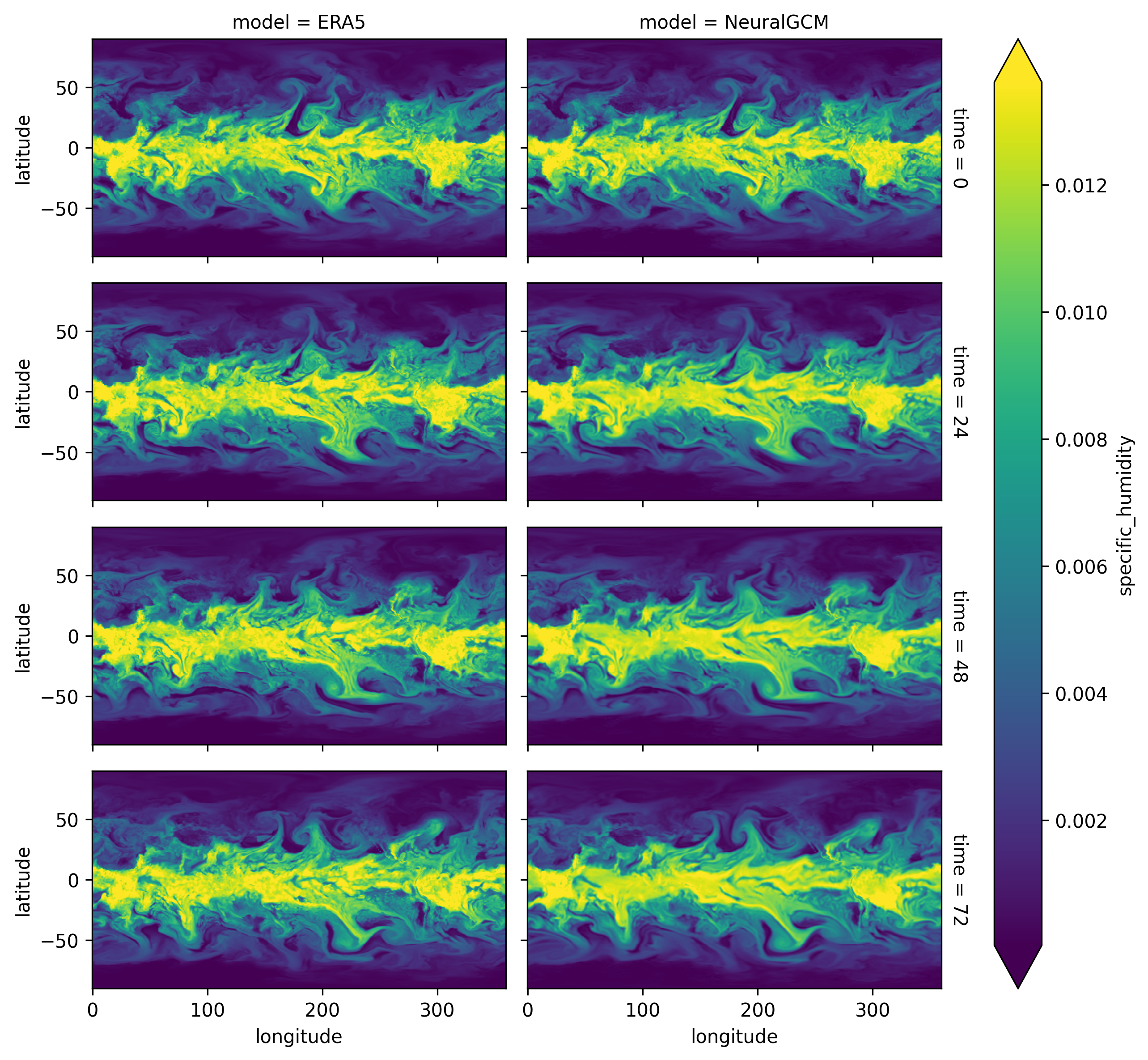
This figure presents the comparison between NeuralGCM's predicted humidity levels and ERA5 ground truth data for a 4-day forecast period. — Fig. 1 NeuralGCM’s predicted humidity level compared to ERA5 ground truth data.#

As we can see, the predicted outputs of NeuralGCM are quite similar to the ERA5 ground truth data.

We will now repeat the previous steps using the latest precipitation model checkpoint v1_precip/stochastic_precip_2_8_deg.pkl. This model allows the prediction of the precipitation_cumulative_mean and evaporation. After running the forecast, the plots can be created (Fig. 2):

os.makedirs('./plots', exist_ok=True)
plot = predictions_ds.precipitation_cumulative_mean.sel(surface=1, time=[24, 48, 72]).plot(
    x='longitude', y='latitude', row='time', robust=True, aspect=2, size=2
)
plot.fig.savefig('./plots/precipitation_cumulative_mean.png', dpi=300, bbox_inches='tight')

plot = predictions_ds.evaporation.sel(surface=1, time=[24, 48, 72]).plot(
    x='longitude', y='latitude', row='time', robust=True, aspect=2, size=2
)
plot.fig.savefig('./plots/evaporation.png', dpi=300, bbox_inches='tight')

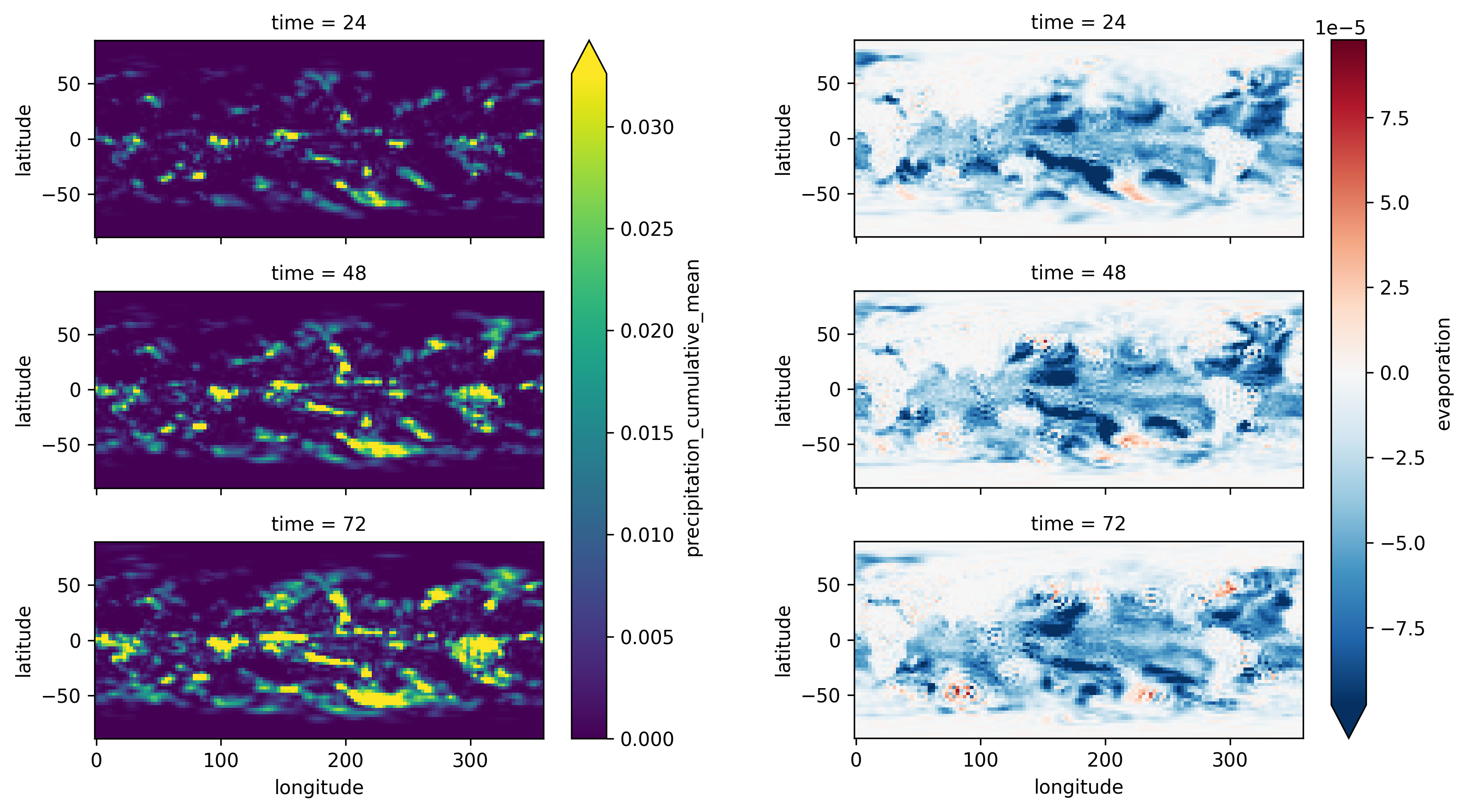
This figure shows the predicted precipitation cumulative mean and evaporation of NeuralGCM precipitation model — Fig. 2 NeuralGCM’s predicted precipitation cumulative mean and evaporation.#

In the above figure, we can see that most of the evaporation is concentrated over oceanic regions, which are represented by negative values, since evaporation is treated as a downward flux in the ERA5 dataset. However, precipitation exhibits a more stochastic and ‘patchy’ distribution. This reflects the complex, non-linear atmospheric processes that govern rainfall.

All of the above inference and plotting code can also be found in this script.

Summary#

In this blog post, we have briefly outlined the challenges of traditional GCMs for weather and climate. We also discussed the difficulties in recent ML-based weather models and hybrid GCMs. We then presented NeuralGCM, explained the basics of how the model works and how it can solve some of these problems. Finally, we showed how one can easily and efficiently run NeuralGCM on AMD Instinct GPU Accelerators and demonstrated how the predictions can be visualized.

Stay tuned for upcoming entries in our weather prediction blog series. We will further investigate other hybrid GCMs when running on AMD hardware. Furthermore, when fluid dynamics equations are discretized on a grid, computational costs scale rapidly with resolution. Researchers are usually forced to choose a grid resolution that is too coarse to simulate small-scale processes, which are then incorporated using ‘subgrid’ models. The use of ML to develop these models has become a prominent area of exploration and will be addressed in the next blog post.

Acknowledgments#

During the writing, the author benefited from helpful comments from and discussions with Rahul Biswas, Luka Tsabadze, Pauli Pihajoki, Sopiko Kurdadze and Baiqiang Xia.

We use software, checkpoints and data contributed by several research groups. We gratefully acknowledge the following:

NeuralGCM by Google®, with resources available at this user manual and in two papers [5], [6]
ERA5 dataset by the European Centre for Medium-Range Weather Forecasts (ECMWF)

References#

[1] Bauer, P., Thorpe, A. & Brunet, G. The quiet revolution of numerical weather prediction. Nature 525, 47–55 (2015)

[2] Hersbach, H. et al. The ERA5 global reanalysis. Quarterly Journal of the Royal Meteorological Society 146, 1999–2049 (2020)

[3] Lam, R. et al. Learning skillful medium-range global weather forecasting. Science 382, 1416–1421 (2023)

[4] Bi, K. et al. Accurate medium-range global weather forecasting with 3d neural networks. Nature 619, 533–538 (2023).

[5] Yuval, J. et al. Neural general circulation models optimized to predict satellite-based precipitation observations. 2412.11973

[6] Kochkov, D. et al. Neural General Circulation Models for Weather and Climate. 2311.07222

[7] Huffman, G. J. et al. Integrated multi-satellite retrievals for the global precipitation measurement (gpm) mission (imerg). Satellite precipitation measurement: Volume 1 343–353 (2020)

[8] Daley, R. Normal mode initialization. Rev. Geophys. 19, 450–468 (1981)

[9] Price, I. et al. Probabilistic weather forecasting with machine learning. Nature 2025, 637, 84–90.

Trademark Attribution#

Docker and the Docker logo are trademarks or registered trademarks of Docker, Inc.

Google is a registered trademark of Google LLC.

Disclaimers#

Third-party content is licensed to you directly by the third party that owns the content and is not licensed to you by AMD. ALL LINKED THIRD-PARTY CONTENT IS PROVIDED “AS IS” WITHOUT A WARRANTY OF ANY KIND. USE OF SUCH THIRD-PARTY CONTENT IS DONE AT YOUR SOLE DISCRETION AND UNDER NO CIRCUMSTANCES WILL AMD BE LIABLE TO YOU FOR ANY THIRD-PARTY CONTENT. YOU ASSUME ALL RISK AND ARE SOLELY RESPONSIBLE FOR ANY DAMAGES THAT MAY ARISE FROM YOUR USE OF THIRD-PARTY CONTENT.

Attribution#

Certain figures (Fig.1, Fig.2) in this post were generated using the NeuralGCM model checkpoints, which are licensed under the Creative Commons Attribution ShareAlike 4.0 International (CC BY SA 4.0) license. Redistribution of these figures should follow the same CC BY SA 4.0 license criteria.