Ensemble High-Resolution Weather Forecasting on AMD Instinct GPU Accelerators#

Weather prediction is fraught with uncertainty, as is the inference of any real-world phenomena dependent on physical observations. The consequence is that any estimated current state of the atmosphere as well as any forecast both carry a level of uncertainty. As such, any weather forecasting model, whether AI or traditional, needs to produce reasonable outputs despite the inherent uncertainty of inputs, and, if possible, quantify the uncertainty of the outputs for the user in some practical fashion.
While theoretically fundamental and thus in principle exactly correct ways to achieve this are known, these are typically not feasible due to computational reasons. However, a common approximate method to tackle the problem in both AI and traditional weather forecasting models has been ensembling.
In ensembling, instead of a single current or forecasted atmospheric state, we use a number of states, slightly different from each other, called an ensemble. This ensemble should then be distributed in a manner that captures both the amount and the precise fashion of our uncertainty about the state of the atmosphere. In machine learning, the ensembles are often generated using so-called generative AI methods. A particularly widely used generative AI method in the weather forecasting industry is the diffusion model.
In this blog post, we will briefly discuss the reasoning for using generative AI models when confronting uncertainty, and outline how diffusion models work. We further describe how high quality predictions can be obtained from an ensemble of forecasts. As an example of a generative weather forecasting model based on diffusion we will use StormCast, a high-resolution convection-allowing model by NVIDIA that we introduced in a previous blog post.
We also provide scripts and step-by-step instructions with which you can get your own StormCast ensemble predictions running and visualized on your AMD Instinct GPUs in no time at all.
Uncertainty in Weather Forecasting#
In weather forecasting, we start from some estimated state of the atmosphere either locally or globally. This state is then propagated forwards using either physical equations or a machine learning model to obtain a forecast. However, there is a large amount of uncertainty in this process.
Firstly, the initial state cannot be known precisely. The measurements of the atmospheric quantities such as temperature, precipitation and wind are not complete, as in that we do not know the values of these quantities everywhere in the atmosphere. The measurements are also not exact, but come with an unavoidable measurement error.
Since the initial state is not known exactly, the forecast consequently cannot be exact either. This is so even if we could solve the atmospheric physics forward in time exactly. As it is, our physical models are not exact either, since we have to make some assumptions in order to be able to calculate the solution with our finite resources. Common approximations in weather forecasting have to do with convection and turbulence, as typical computational grids may be too coarse to resolve these phenomena. While machine learning models may offset some of these difficulties, they do not provide exact propagation either.
The end result is that we start with an uncertain state and propagate it using methods that can only add to this uncertainty. How can this state of affairs be managed? In principle, we can represent the resulting uncertainty of the forecast as a distribution, and compute it to arbitrary (numerical) precision through a full Bayesian computation. However, this is typically computationally unfeasible. Instead, computational shortcuts like ensembles are used to represent the distribution of the forecast, and these ensembles are often created using generative AI methods such as diffusion models.
Generative models#
In short, generative models are models with which we can straightforwardly generate new examples \(x\) of data from some distribution of interest \(p(x)\). This is in contrast to discriminative models, which can only represent the conditional probability \(p(y|f(x))\) of a particular output \(y\) given some input data \(x\) and the model function \(f\).
In this condensed, probabilistic formulation the generative approach sounds simple and straightforward. However, in practice, the desired distribution of data to be generated may be high-dimensional, utterly convoluted, hard to quantify, and possibly only available through learning from data. This also makes sampling from the distribution a complex and demanding task.
One recent approach to this problem is a family of models called diffusion models. This is also the approach used by StormCast to generate its predictions and ensembles.
Diffusion models#
Overview#
The main idea of diffusion models is as follows: Since our target distribution may be computationally infeasible to estimate and to sample from, we instead sample from an “easy” alternative distribution and learn a method that transforms our sample to a sample of the desired distribution, possibly gradually in small steps.
An obvious alternative distribution is the normal distribution, i.e. the Gaussian noise distribution. A diffusion process will turn any distribution into a Gaussian noise distribution, and it is possible to learn an inverse process using data. To generate new data from the target distribution, we can then simply sample from a normal distribution, optionally with conditioning, and then apply the inverse process.
Why diffusion models work#
The technical basis of why this works rests on a few key results. We define the diffusion process as a Gaussian noise model
where \(q(x_t|x_{t-1})\) is the transition probability density, \(x_t\) is a sample from our target distribution after \(t\) steps of the diffusion process (also called latent state), \(\beta_t\) is a noise schedule, \(I\) is the identity matrix and \(\mathcal{N}\) is the normal distribution. With this choice, we can have a direct analytic solution for the transition probability from the initial sample to the latent state at any \(t\) with
where \(\alpha_t = 1-\beta_t\) and \(\bar{\alpha}_t = \alpha_1 \cdots \alpha_t\).
This distribution \(q(x_t|x_0)\) is called the diffusion kernel, and with it we can directly write the noisy distribution \(q\) at any \(t\) via
where \(q_0\) is our original target distribution. From this we can show that when \(t\) increases, the resulting distribution becomes increasingly like pure Gaussian noise.
These results show that we can efficiently create progressively noisy samples for training purposes, but they also hint at the inverse process. In fact, if we knew \(x_0\), we could directly invert the diffusion process using standard Bayesian methods, and obtain
where \(\tilde{\mu}(x_t,x_0)\) is a bilinear function and \(\tilde{\beta}\) a function of \(\beta_t\) only.
However, during inference we don’t actually know \(x_0\), but only \(x_T\) sampled from the noise distribution. Instead, \(x_0\) is what we would like to obtain. Thus we write the inverse process as
where \(\mu_{\theta}\) and \(\Sigma_{\theta}\) are parametrized mean and covariance models we will learn from the data. With this approach we can now sample an \(x_T\) from the noise distribution \(\mathcal{N}(0,I)\) and denoise it using our learned inverse process.
Diffusion models based on the simple prescription described above are commonly known as the Denoising Diffusion Probabilistic Models (DDPM), and form the basis of the model used in StormCast. However, the diffusion model family has grown immensely in just the past few years, and it is recommended to see, for example, [1] for a recent survey of the field.
Generative modelling and ensembles in StormCast#
For an overview of the StormCast model structure it is recommended to read our previous blog post on the model, as well as the original publication [2]. In short, StormCast first uses a deterministic model to predict a mean atmospheric state. It then uses a particular diffusion model, i.e. a generative method to sample a residual, which when added to the mean state produces a sample from the estimated distribution of possible forecasted atmospheric states.
To create skillful forecasts, this generative modelling is combined with ensembling. What this means in practice is that a number of copies or an ensemble of the same initial state is created. These copies are then individually fed through the StormCast forecasting model. When the copies enter the generative part, they each get assigned a different sampled residual, which causes the ensemble members to diverge. This also results in the ensemble modelling the target distribution of the forecasted weather states in a probabilistic fashion.
This probabilistic ensemble can then be used to compute more detailed forecasts. Firstly, each ensemble member is a different possible realization of the forecasted weather and when visualized provides an immediate, visual feedback on both likely weather and the degree of uncertainty of the estimate. It can also be used to compute various derived estimates such as the Probability Matched Mean (PMM) used in the original StormCast publication.
In the tests run by the authors, StormCast was compared to the state-of-the-art traditional forecasting system High-Resolution Rapid Refresh (HRRR) developed and maintained by the National Oceanic and Atmospheric Administration (NOAA). The authors found that both the individual StormCast ensemble member forecasts as well as the PMM estimates were as accurate as the HRRR forecasts, and superior on shorter timescales.
StormCast diffusion model#
The core of the diffusion model used by StormCast is the denoiser architecture the authors call DDPM++ U-Net, originally formulated in [3]. This approach follows the outline given above, but with an U-Net neural network used as the basis for the inverse diffusion process.
The diffusion model is trained on the residuals \(r_{t+1} = M_{t+1}-\mu_{t+1}\) between the (known) meso-scale states \(M_{t+1}\) and the predicted mean states \(\mu_{t+1}\). For a description of how the mean states are predicted, see the previous blog post in our series.
During inference, the model is then used to sample a residual \(r_{t+1}\) from the conditional probability distribution \(p(r_{t+1}|\mu_{t+1},M_t,S_t)\), where \(\mu_{t+1}\) is again the predicted mean state, and \(M_t\) and \(S_t\) are the currently known meso-scale and synoptic scale states. This conditioning is achieved by concatenating all these values into one high-dimensional vector \(c\), which can then be concatenated with the original argument \(x\), which essentially forces the model to learn from pairs \((x,c)\). The resulting residual \(r_{t+1}\) is then added to the mean estimate \(\mu_{t+1}\) to form the full estimate of the future meso-scale state \(M_{t+1}\).
During computation, as long as the random number generator state is not duplicated, the residuals \(r_{t+1}\) will be independent samples. This makes it possible to initiate an ensemble from a single mean state estimate \(\mu_{t+1}\) simply by sampling the residual as many times as desired. The resulting ensemble will then automatically conform to the estimated distribution \(p(M_{t+1}|M_t,S_t)\) of future meso-scale states \(M_{t+1}\) given the current meso-scale and synoptic scale states \(M_t\) and \(S_t\), respectively.
The process described above is how StormCast uses diffusion for prediction and for initiating ensembles. However, it should be noted that during inference the ensemble, once generated, is then passed through the inference process without generating any additional samples. That is, StormCast does not generate a set of new ensemble members for each pre-existing member during each prediction step, as this would lead to an exponential increase of the size of the ensemble.
Using an ensemble for prediction#
With an ensemble of predictions of the future meso-scale atmospheric state \(M_{t+1}\) available, a natural question arises: How should this ensemble best be used for reasoning about the future? If the model is well calibrated, the members of the ensemble should all be possible future weather states, if not all equally likely, since they are all samples of the learned conditional distribution \(p(M_{t+1}|M_t,S_t)\) (see above). So which one, if any, is the best prediction?
One might think that computing the ensemble mean ought to be a good choice, perhaps pondering the fact that the empirical mean minimizes the root mean square error (RMSE). However, if we consider the limit of an infinitely large ensemble, which one might think would also increase the faithfulness of the ensemble approximation, the ensemble mean in StormCast’s case is just the predicted mean state \(\mu_{t+1}\) again. This is retrospectively obvious, since the deterministic part of StormCast was explicitly trained to predict this future mean.
Even aside from this, the ensemble mean, while possibly producing improvements with respect to metrics like RMSE, may produce large errors in other quantities such as bias or extremal values [4]. This has to do with the fact that the ensemble mean emphasizes highly predictable features that the ensemble members agree on, but averages out features that are more difficult to predict. This in effect suppresses high-frequency content, contracts the range of output values and generally produces outputs that have a smoothed appearance. This tendency has led to the development of alternative ways to combine the ensemble information that work better for these kinds of quantities. One of these methods is called the Probability Matched Mean (PMM), mentioned above in passing.
Probability Matched Mean (PMM)#
The fundamental idea of PMM is to replace the list of sorted values of the ensemble mean with the pooled, sorted and decimated list of values of the entire ensemble, where value refers to any predicted quantity [4]. This has the effect of counteracting the range-contracting and smoothing tendencies of the ensemble mean. The replacement can be done either by using the pooled ensemble globally, or only locally within some specified range of each gridpoint. The latter approach is referred to as the localized PMM [5].
In practice the original global method (originally from [4], but the version from [5] is presented here) works in the following manner for a given predicted quantity, over an ensemble of \(n\) members:
Compute the ensemble mean \(\bar{A}\) of the quantity \(A\) over all grid points \(x_i\in X\) to create the list \(h=\{\bar{A}(x_i)|x_i\in X\}\)
Sort the resulting list \(h\) of values in ascending order, keeping track of which grid point each value belongs to.
Pool all values of the quantity over all \(n\) ensemble members and grid points to create the list \(g=\{A_1(x_i),\ldots,A_n(x_i)|x_i\in X\}\). Sort in ascending order.
From the list \(g\) of ensemble member values drop all but every \(n\)’th value. This yields a list of values equal in length to the list \(h\) of ensemble mean values.
Replace each value in the ensemble mean list \(h\) by the corresponding value in the ensemble member list \(g\).
In Python code, the procedure above translates to the following function
definition, assuming the input is an xarray.DataArray object. This is also
the implementation used in the plot-stormcast.py
program provided with this blog post. Note that here descending sorts are used,
as in the original definition
given in [4].
def pmm(arr: xr.DataArray):
    # Get ensemble size.
    n_ens = arr.sizes['ensemble']

    # Then compute the ensemble mean at every gridpoint.
    ens_mean = arr.mean(axis=0)
    np_mean = ens_mean.to_numpy()

    # Also create flattened index arrays into the ensemble mean array.
    ys, xs = np_mean.shape
    ymat, xmat = np.mgrid[0:ys, 0:xs]
    y_flat = ymat.flatten()
    x_flat = xmat.flatten()

    # Next, argsort the flattened ensemble mean, descending. Use these incides to sort the flattened index arrays.
    sorted_ix = np.argsort(np_mean.flatten())[::-1]
    y_sorted = y_flat[sorted_ix]
    x_sorted = x_flat[sorted_ix]

    # Pool all ensemble values across every grid point, sort descending and keep
    # every n'th, where n is the number of members in the ensemble.
    ens_sorted_desc = np.sort(arr.to_numpy().flatten())[::-1]
    ens_sorted = ens_sorted_desc[::n_ens]

    # Update the ensemble mean values from the pooled and sorted ensemble values to create the PMM.
    updated_mean = ens_mean.copy()
    np_updated = np.zeros_like(np_mean)
    np_updated[y_sorted, x_sorted] = ens_sorted
    updated_mean.values = np_updated

    # Return the result as a DataArray.
    return updated_mean
As described in [4], the PMM procedure essentially takes in an ensemble mean, keeps the correlation between the sorted rank and spatial location intact, but replaces the value of the quantity with the value of the corresponding rank from the list of pooled and sorted ensemble member values. This in effect changes the implied probability distribution of the input ensemble mean to match the probability distribution of the entire pooled set of ensemble member values. As such, especially the extremal values in the pooled ensemble will now be present in the result. However, the procedure is rather ad hoc in nature, and has some disagreeable characteristics.
For example, when picking every \(n\)’th value from the pooled list of ensemble member values, we get the sequence of \((n,2n,3n,\ldots,Mn)\), where \(M\) is the number of gridpoints. This sequence contains the smallest value from the pooled list, at position \(Mn\), but not the largest. Likewise, if we start by taking the first value, so the sequence \((1,n+1,2n+1,\ldots,(M-1)n+1)\), the sequence contains the largest value, but not the smallest. Hence there is a degree of freedom in what the output is, and the choice may vary by implementation. For example [4] and [5] sort the values by descending and ascending order respectively, which produce different results even for the same sequence of every \(n\)’th value chosen.
The localized PMM is slightly different, using the following process (from [5]):
Compute the ensemble mean over all gridpoints, as in the global method.
Within a given radius \(\rho\) of each grid point sort the ensemble mean values in ascending order and note the rank \(R_m\) of the value corresponding to the grid point.
Within the same radius \(\rho\) of each grid point, pool all the ensemble member values and sort in ascending order.
Replace the ensemble mean value at the grid point by the value from the list of ensemble member values corresponding to the rank \(R_e=nR_m\).
This change has the effect of limiting the range of PMM procedure affecting the value at each gridpoint spatially to some maximum range \(\rho\). This method now has a further degree of freedom in the choice of \(\rho\). In addition, the reference [5] proposes more involved, empirically based choices for determining \(R_e\) from \(R_m\), but these are even more ad hoc and not guaranteed to produce good results for other datasets than the particular one used in the publication.
Despite the problems mentioned above, the PMM algorithm is an often used tool in the weather prediction field, and works well there. As such, we will show below how the PMM can be plotted for any StormCast ensemble output.
Installing StormCast#
As prerequisites, you will need the following at a minimum:
A computer with an AMD Instinct GPU. The examples in this blog post were run on an MI300X.
A GNU/Linux operating system with Docker installed.
ROCm kernel driver installed. See the instructions for running ROCm Docker containers.
We have covered the rest of the installation instructions in the previous blog post, and we recommend you follow the directions there.
Note
We have updated the scripts for running and plotting ensemble forecasts, so you will need to download these updated versions: run-stormcast.py and plot-stormcast.py. Save these into your working directory from which you launch your Docker container as specified in the instructions.
Running inference#
Using Earth2studio, running the StormCast ensemble forecasts happens nearly identically to running the non-ensemble forecasts. For reference, we can launch a non-ensemble forecast for a given number of forecasting steps using the following:
import earth2studio.run as run
from earth2studio.models.px import StormCast
from earth2studio.data import HRRR
from earth2studio.io import ZarrBackend
from datetime import datetime

package = StormCast.load_default_package()
model = StormCast.load_model(package)
data = HRRR()
io = ZarrBackend('model-output.zarr')
starting_datetime = datetime(year=2025, month=8, day=9, hour=12)
nsteps = 12
io = run.deterministic(time=[starting_datetime], nsteps=nsteps, prognostic=model, data=data, io=io)
For an explanation of what all of the preliminaries do, please refer to the previous blog post.
To change this to run an ensemble forecast instead, it is sufficient to change the runner function and provide information about the number of ensemble members as well as their initialization. This can be achieved by replacing the last line of the above snippet with the following:
from earth2studio.perturbation import Zero
nensemble = 4
io = run.ensemble(time=[starting_datetime], nsteps=nsteps, nensemble=nensemble,
                  prognostic=model, data=data, io=io, perturbation=Zero())
Here, nensemble specifies the number of members to be included in the ensemble,
here four. The perturbation parameter on the other hand, specifies the ensemble
member initialization through specifying the kind of perturbation that should be
applied to the initial state to obtain the ensemble. As discussed above,
StormCast will naturally separate the ensemble members from each other through
the random sampling of the residual distribution, and as such the Zero
perturbation (i.e. no perturbation at all) is used here.
Running the code above will run a StormCast ensemble of four members and
propagate each for twelve timesteps of one hour. The result is a zarr output (which
on the disk is stored as a directory hierarchy) containing the forecasts for
each ensemble member.
An easier way to run StormCast in ensemble mode is to use the StormCast runner program run-stormcast.py we have provided. Using the program the above result can be achieved by running the following:
python run-stormcast.py --ensemble --ensemble-size 4 2025-08-09T12:00 12
This will perform the exact same run, but is much easier to use. Try using the
--help command line argument to get additional information on how to use the
program.
The output structure#
The output is a zarr store, which will have the following coordinates:
ensemble: Indexes through ensemble members, from 0 tonensemble-1.time: The date and time of the initial state, as adatetime64[ns].lead_time: The lead time of the initial state (which is 0) and each forecast step, as atimedelta64[h]. Will have a size ofnsteps+1.hrrr_y: The native projected HRRR \(y\)-coordinate.hrrr_x: The native projected HRRR \(x\)-coordinate.
The forecasted quantities are stored as data variables, with most using the
format [varname][vertical-level]hl for hybrid-sigma vertical levels and
[varname][height-level] for a height level. As such, u10hl would be the wind
\(u\)-component predicted for the 10th hybrid-sigma vertical level, and u10m
would be the wind \(u\)-component predicted at the height of 10 meters. In
addition there are some specific variables such as refc for the composite
radar reflectivity.
Thus, in order to for example compute the ensemble mean radar reflectivity for the 4th timestep we could do the following:
data = ds['refc']
ensemble_mean = data[:,0,4].mean(axis=0)
Here we assume that ds contains the zarr output.
In general for ideas on how to manipulate the output data, we suggest taking a look inside the plot-stormcast.py plotting program, which we will be using below to plot the results.
Plotting#
Ensemble runs have a much larger selection of quantities one might be interested in plotting, such as all the ensemble members and different ensemble means or other collective quantities. We have expanded the plot-stormcast.py program to showcase some of the possibilities you might be interested in.
In its upgraded form it will automatically detect when given an ensemble run to plot, and will then plot each timestep as a three rows by two columns plot with the following panels (from left to right, top to bottom):
The HRRR forecast.
The HRRR analysis data (used as ground truth).
One StormCast ensemble member (specified as a command line argument).
The StormCast probability matched mean (PMM).
The StormCast ensemble mean.
An error plot giving the RMSE errors of the HRRR forecast and the StormCast PMM and ensemble means.
As an example, to plot the composite radar reflectivity (the default choice) for the ensemble run shown above you would do the following:
python plot-stormcast.py outputs/pred-2025-08-09.zarr
This will plot all the frames and save them into the working directory with names
scast-2025-08-09-refc-[frame-number].jpg, where [frame-number] is the index
of the timestep. See Figure 1 below for an example output.
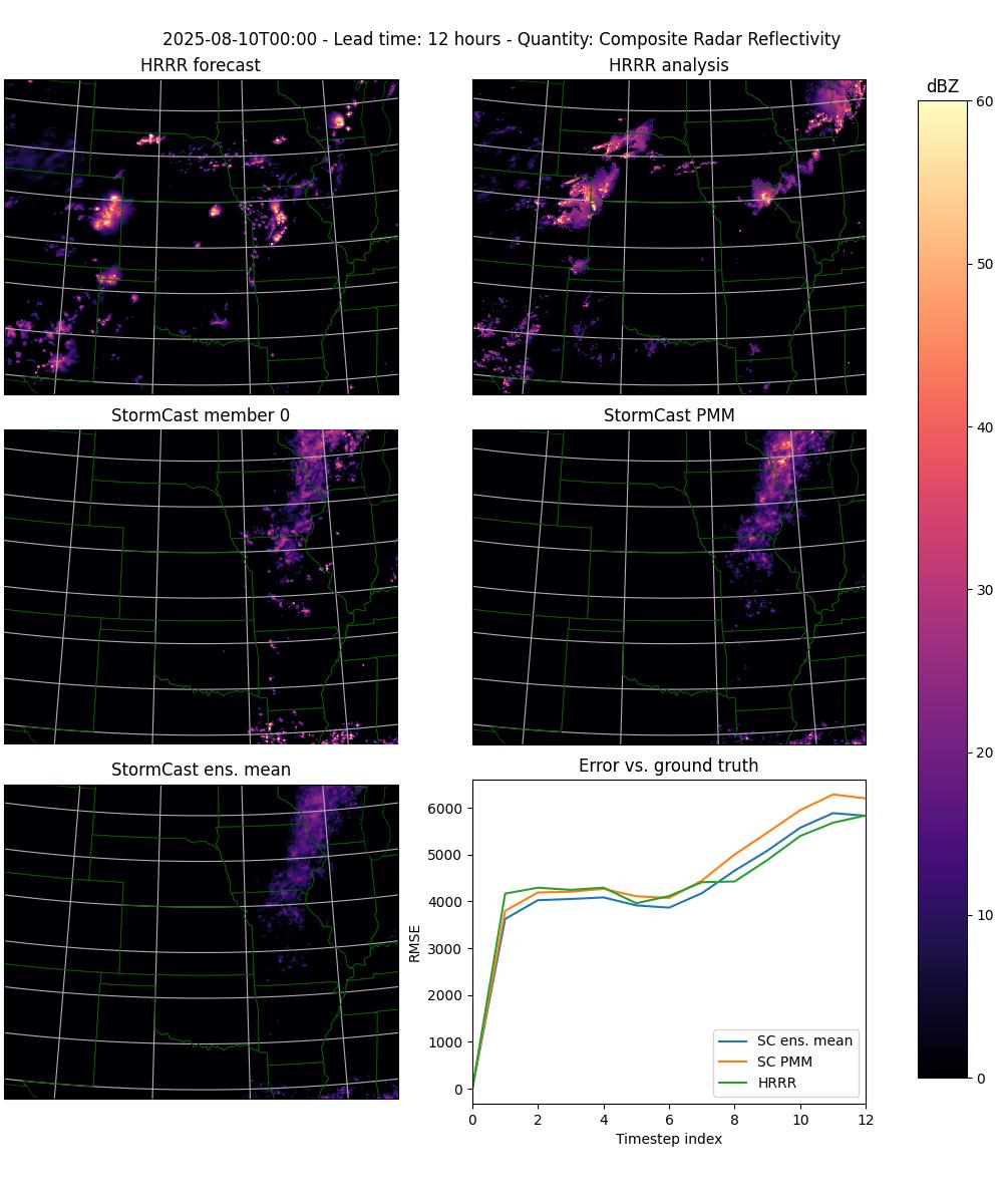
Figure 1. Frame 12 from the sequence of frames produced with the plot-stormcast.py program.#
If you have ImageMagick installed on your system, you can easily turn these into an animated gif by running the following:
convert -loop 0 -delay 100 scast-2025-08-09-refc-*.jpg animation.gif
This will produce an animated gif that will loop endlessly with a one-second delay
between the frames, saved as the file animation.gif. See Figure 2 below for an
example.
Figure 2. An animation of the frames plotted by the plot-stormcast.py program.#
To plot different quantities, you can use the --quantity command line
argument. Currently only refc (composite radar reflectivity) and t2m
(temperature at the height of two meters) are supported, but the code is laid
out so that you can easily extend this to your liking. Also try the --help
command line parameter to see all the other options and further help on how to
use the program.
Summary#
Competent forecasting of physical phenomena, such as weather, requires explicit and skillful management of uncertainty. One way to represent uncertainty is through ensembles, where the distribution of the elements in the ensemble represents the uncertainty of the forecast. In machine learning, an interesting possibility for constructing ensembles is by leveraging diffusion models. These models can sample new examples of data from any complicated distribution by a clever sleight of hand: learning a process that correlates a noise distribution to the desired data distribution, and then sampling from the simple noise distribution instead.
In this blog post we have outlined how uncertainty can be incorporated using a particular subset of generative AI, namely diffusion models. We have described how diffusion is used in StormCast, a particular weather prediction model, to build ensembles capturing the uncertainty of the predictions. In addition, we described how these ensembles can be leveraged to create enhanced predictions through ensemble means and probability matched means.
Lastly, we demonstrated how high-resolution ensemble weather prediction can be easily run on AMD Instinct GPUs. We showcased this using the StormCast model and our example Python programs. These programs make it easy and straightforward to both run the StormCast model in ensemble mode and to plot the resulting forecasts.
If you’ve enjoyed this blog post, please do check out our other blog posts in our weather prediction series. We have previously covered topics such as running synoptic scale models, training a synoptic scale model, as well as high-resolution forecasting. Be on the lookout for forthcoming blog posts in this series as well!
Acknowledgments#
The author acknowledges helpful discussions with Rahul Biswas, Sopiko Kurdadze, and Luka Tsabadze.
Additional Resources#
The StormCast runner program: run-stormcast.py
The StormCast plotter program: plot-stormcast.py
License#
StormCast comes bundled with Earth2Studio, released under the Apache License 2.0. Please see the full text of the license.
References#
[1] Shen, H. et al. (2025). Efficient Diffusion Models: A Survey. arXiv:2502.06805
[2] Pathak, J., Cohen, Y., Garg, P., Harrington, P., Brenowitz, N., Durran, D., Mardani, M., Vahdat, A., Xu, S., Kashinath, K., Pritchard, M. (2024). Kilometer-Scale Convection Allowing Model Emulation using Generative Diffusion Modeling. arXiv:2408.10958. https://arxiv.org/abs/2408.10958.
[3] Song Y. et al. (2021). Score-Based Generative Modeling through Stochastic Differential Equations. International Conference on Learning Representations. arXiv:2011.13456.
[4] Ebert, E. (2001). Ability of a Poor Man’s Ensemble to Predict the Probability and Distribution of Precipitation. Mon. Wea. Rev., 129, 2461–2480. https://doi.org/10.1175/1520-0493(2001)129<2461:AOAPMS>2.0.CO;2.
[5] Clark, A. J. (2017). Generation of Ensemble Mean Precipitation Forecasts from Convection-Allowing Ensembles. Wea. Forecasting, 32, 1569–1583, https://doi.org/10.1175/WAF-D-16-0199.1.
Disclaimers#
Third-party content is licensed to you directly by the third party that owns the content and is not licensed to you by AMD. ALL LINKED THIRD-PARTY CONTENT IS PROVIDED “AS IS” WITHOUT A WARRANTY OF ANY KIND. USE OF SUCH THIRD-PARTY CONTENT IS DONE AT YOUR SOLE DISCRETION AND UNDER NO CIRCUMSTANCES WILL AMD BE LIABLE TO YOU FOR ANY THIRD-PARTY CONTENT. YOU ASSUME ALL RISK AND ARE SOLELY RESPONSIBLE FOR ANY DAMAGES THAT MAY ARISE FROM YOUR USE OF THIRD-PARTY CONTENT.