Medical Imaging on MI300X: SwinUNETR Inference Optimization#

This post is the inference companion to our training walkthrough, Medical Imaging on MI300X: Optimized SwinUNETR for Tumor Detection. In this post, we focus on inference latency and throughput for 3D CT segmentation of tumors on MI300X, and we share the two optimizations that delivered the biggest wins in practice:
Automatic Mixed Precision (AMP) via
autocastModel compilation with
torch.compile
With these changes, we observed substantial performance improvements across different ROI sizes while preserving segmentation quality.
SwinUNETR Overview#
SwinUNETR is a transformer-based architecture for 3D medical image segmentation. It combines the Swin Transformer’s ability to capture long-range spatial dependencies with UNETR’s encoder-decoder design, making it particularly effective for volumetric data like CT and MRI scans. For a detailed introduction to the model architecture and training setup, see our companion training blog.
Why Inference Optimization Matters#
In clinical settings, inference speed directly impacts patient care. Radiologists and clinicians need rapid feedback when analyzing medical scans, whether for surgical planning, treatment monitoring, or emergency diagnosis. Optimizing inference is not just about reducing costs, it’s about enabling real-time decision support that can save lives.
Unlike training, where you optimize once and amortize the cost over the model’s lifetime, inference runs continuously in production. Even small latency improvements compound into significant resource savings and better user experiences. For medical imaging workloads processing large 3D volumes, these optimizations are particularly impactful.
Why inference is different#
Training stresses backward ops and benefits from convolution auto-tuning. Inference is dominated by forward compute plus sliding-window tiling (for 3D), so the fastest path comes from:
Reducing math cost (use AMP where numerically safe)
Specializing kernels and fusing graphs (
torch.compile)Feeding the GPU efficiently (right ROI, right
sw_batch_size, and warm workers)
On recent ROCm/PyTorch releases, forward convolutions are well-optimized and performant without requiring much additional tuning. The levers that moved the needle the most for SwinUNETR inference were autocast and torch.compile.
Inference Optimization Techniques#
We evaluated two primary optimization strategies available in PyTorch that require minimal code changes and provide substantial performance improvements on AMD hardware.
Automatic Mixed Precision with Autocast#
PyTorch’s autocast context manager automatically selects the optimal precision for different operations during inference. It intelligently downcasts operations like matrix multiplications and convolutions to FP16, while keeping precision-sensitive operations like reductions in FP32.
For inference workloads, autocast provides several benefits:
Reduced memory bandwidth requirements by processing data in lower precision
Better cache locality due to smaller data footprints
Potential utilization of specialized hardware units optimized for FP16 operations
The implementation is straightforward:
import torch
from monai.networks.nets import SwinUNETR

# Load your trained model
model = SwinUNETR(
    img_size=(96, 96, 96),
    in_channels=1,
    out_channels=1,
    feature_size=48
)

model_dict = torch.load("model.pt", weights_only=False)["state_dict"]
model.load_state_dict(model_dict)
model.eval()
model.to("cuda")

# Perform inference with autocast
with torch.inference_mode():
    with torch.autocast(device_type="cuda", dtype=torch.float16, dynamic=False):
        output = model(input_tensor)
Autocast automatically handles precision casting without requiring manual intervention, making it an ideal first optimization step.
Torch.compile#
PyTorch 2.0 introduced torch.compile, a Just-In-Time (JIT) compiler that transforms PyTorch code into optimized kernels tailored for specific hardware. The compiler performs several advanced optimizations:
Kernel fusion: Combines multiple operations to reduce memory transfers and launch overhead
Memory access optimization: Improves cache locality through tiling and layout transformations
Shape specialization: Tailors computations precisely to model dimensions
We use the mode="max-autotune" setting for compilation, which performs the most extensive optimization search, allowing PyTorch to automatically select the fastest kernel implementations for each operation.
Implementation requires just a single line of code:
# Compile the model with max-autotune for peak performance
model = torch.compile(model, mode="max-autotune")

# Warmup: trigger compilation with representative inputs
with torch.inference_mode():
    _ = model(warmup_input)

# Inference
with torch.inference_mode():
    output = model(input_tensor)
Torch.compile is a JIT compiler, meaning the first inference triggers compilation. This initial compilation can take several minutes depending on model complexity. For production deployments:
Use compilation caching to reduce startup time when launching new instances
Always warmup inference processes with representative inputs before serving production traffic
Benchmarks#
We measured end-to-end average inference time per sample (lower is better) across three ROI sizes. All runs used identical preprocessing, and the sliding window batch size was tuned for optimal throughput in each configuration.
For these benchmarks, we used the same SwinUNETR codebase as in the previous training blog post, but with the latest ROCm v7.0 release available at the time of writing as the base image: rocm/pytorch:rocm7.0_ubuntu24.04_py3.12_pytorch_release_2.6.0
All benchmarks were conducted with MIOpen Auto-Tuning enabled (MIOPEN_FIND_MODE=1, MIOPEN_FIND_ENFORCE=3), which improves inference performance by approximately 15-20% by automatically selecting the most optimal kernels for convolution operations. To learn more about MIOpen Auto-Tuning and how it was used to achieve significant training performance improvements, see our previous training blog post.
Measured Dice scores were consistent across configurations (±2%), with no detectable degradation in accuracy compared to the baseline, confirming that the numerical precision changes introduced by autocast AMP (FP16) and the optimizations from torch.compile did not negatively impact segmentation quality.
Time per case (lower is better)#
Table 1 summarizes the inference time for each optimization configuration across three ROI sizes, measured as average seconds per sample. For consistency, all configurations within each ROI column use the same sliding window batch size: batch size 12 for 96×96×96, batch size 8 for 128×128×128, and batch size 4 for 256×256×128. These batch sizes were selected based on the optimal performance of the combined autocast + compile configuration.
Config |
ROI 96×96×96 |
ROI 128×128×128 |
ROI 256×256×128 |
|---|---|---|---|
baseline |
4.25s |
4.02s |
3.41s |
autocast |
2.60s |
2.63s |
2.19s |
compile |
3.57s |
3.28s |
2.50s |
autocast + compile |
1.74s |
1.66s |
1.17s |
Table 1. Inference time (seconds per sample) for each configuration.
Takeaways#
Use
autocastandtorch.compiletogether for optimal performance. The combined optimization consistently delivers the best results across all ROI sizes, achieving up to 2.9× faster inference compared to baseline.AMP (
autocast) alone provides reliable speedups of 35–39% across all ROI sizes, making it an excellent first optimization step.
Memory usage#
The sliding window batch size (sw_batch_size) controls how many patches of a single 3D volume are processed in parallel during inference — not the traditional “batch size” used across multiple samples.
Figure 1 shows how memory usage scales with batch size across different optimization configurations.
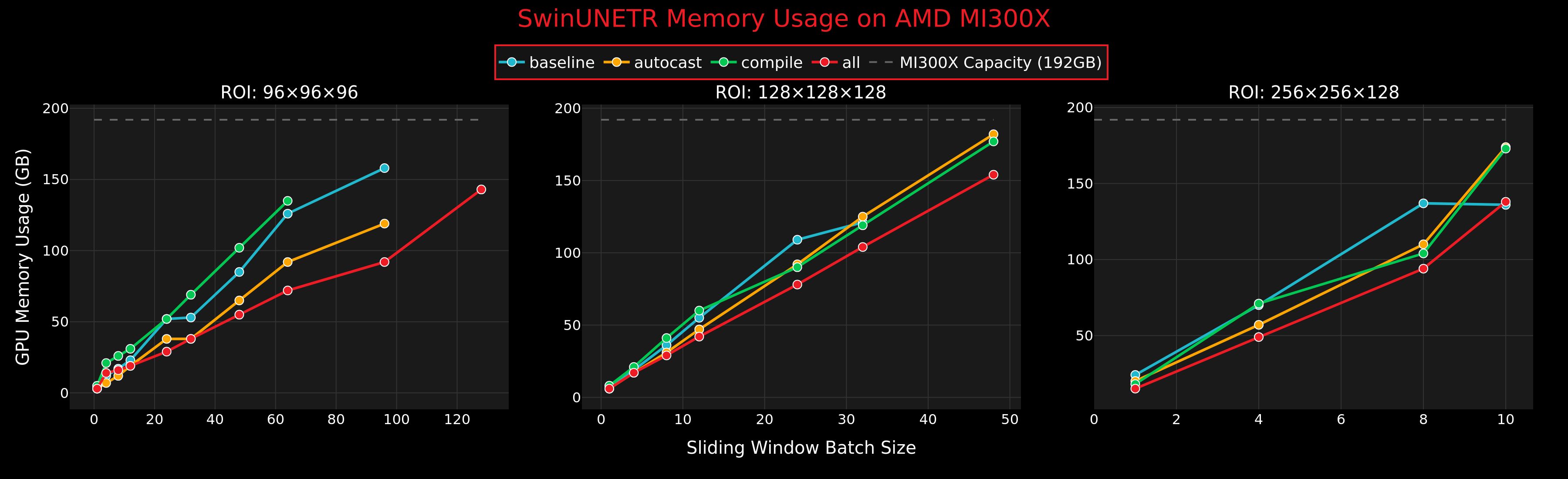
Figure 1. GPU memory usage vs sliding window batch size for SwinUNETR on AMD MI300X across three ROI sizes. The gray dashed line at 192GB indicates MI300X memory capacity.#
Memory Takeaways#
The MI300X’s massive 192 GB memory accommodates large batch sizes even for the biggest ROIs, where most GPUs would be severely constrained.
Autocast significantly reduces the memory footprint through FP16 precision, allowing for larger batch sizes.
Combined optimization delivers both the fastest inference times and the most efficient memory usage, reducing memory footprint by ~25%.
Summary#
This blog demonstrated how to optimize SwinUNETR inference on AMD MI300X GPUs using PyTorch’s simple built-in optimization features. By combining automatic mixed precision via autocast and just-in-time compilation via torch.compile with max-autotune mode, we achieved up to 2.9× faster inference compared to baseline performance while maintaining model accuracy.
Key Deliverables#
This blog provides practitioners with:
Practical optimization guide for applying
autocastandtorch.compileto medical imaging inference workloads and getting the best performance out of the MI300X GPUs.Comprehensive benchmarks across multiple ROI sizes demonstrating real world performance gains.
Performance analysis showing how different optimization methods and the large AMD MI300X memory capacity enable scalable, low-latency inference on large 3D volumes.
Disclaimers#
Third-party content is licensed to you directly by the third party that owns the content and is not licensed to you by AMD. ALL LINKED THIRD-PARTY CONTENT IS PROVIDED “AS IS” WITHOUT A WARRANTY OF ANY KIND. USE OF SUCH THIRD-PARTY CONTENT IS DONE AT YOUR SOLE DISCRETION AND UNDER NO CIRCUMSTANCES WILL AMD BE LIABLE TO YOU FOR ANY THIRD-PARTY CONTENT. YOU ASSUME ALL RISK AND ARE SOLELY RESPONSIBLE FOR ANY DAMAGES THAT MAY ARISE FROM YOUR USE OF THIRD-PARTY CONTENT.