Analyzing the Impact of Tensor Parallelism Configurations on LLM Inference Performance#

As AI models continue to scale in size and complexity, deploying them efficiently requires strategic resource allocation. Tensor parallelism (TP) is a valuable technique for distributing workloads across multiple GPUs, reducing memory constraints, and enabling inference for large-scale models. However, the choice of TP configuration isn’t one-size-fits-all—it directly impacts performance, networking overhead, and cost efficiency.
In this blog, we explore the mechanics of tensor parallelism, its impact on throughput and latency across different batch sizes, and the trade-offs between high TP configurations and single-GPU (TP=1) deployments. You’ll discover how TP affects networking overhead, why certain workloads benefit from lower TP values, and how AMD Instinct™ GPUs leverage memory advantages to optimize multi-model hosting. Whether you’re deploying massive LLMs or optimizing inference for cost-sensitive applications, this blog will help you navigate the complexities of TP configurations to maximize AI infrastructure efficiency.
An Introduction to Tensor Parallelism#
Tensor parallelism is a technique supported by most inference frameworks/engines, where the tensors in the neural network are split along the hidden layer dimension and distributed to multiple GPUs to reduce the per-GPU memory and compute burden. The use of multiple GPUs with TP enables larger batch sizes and larger models that normally would not fit into a single GPU’s memory.
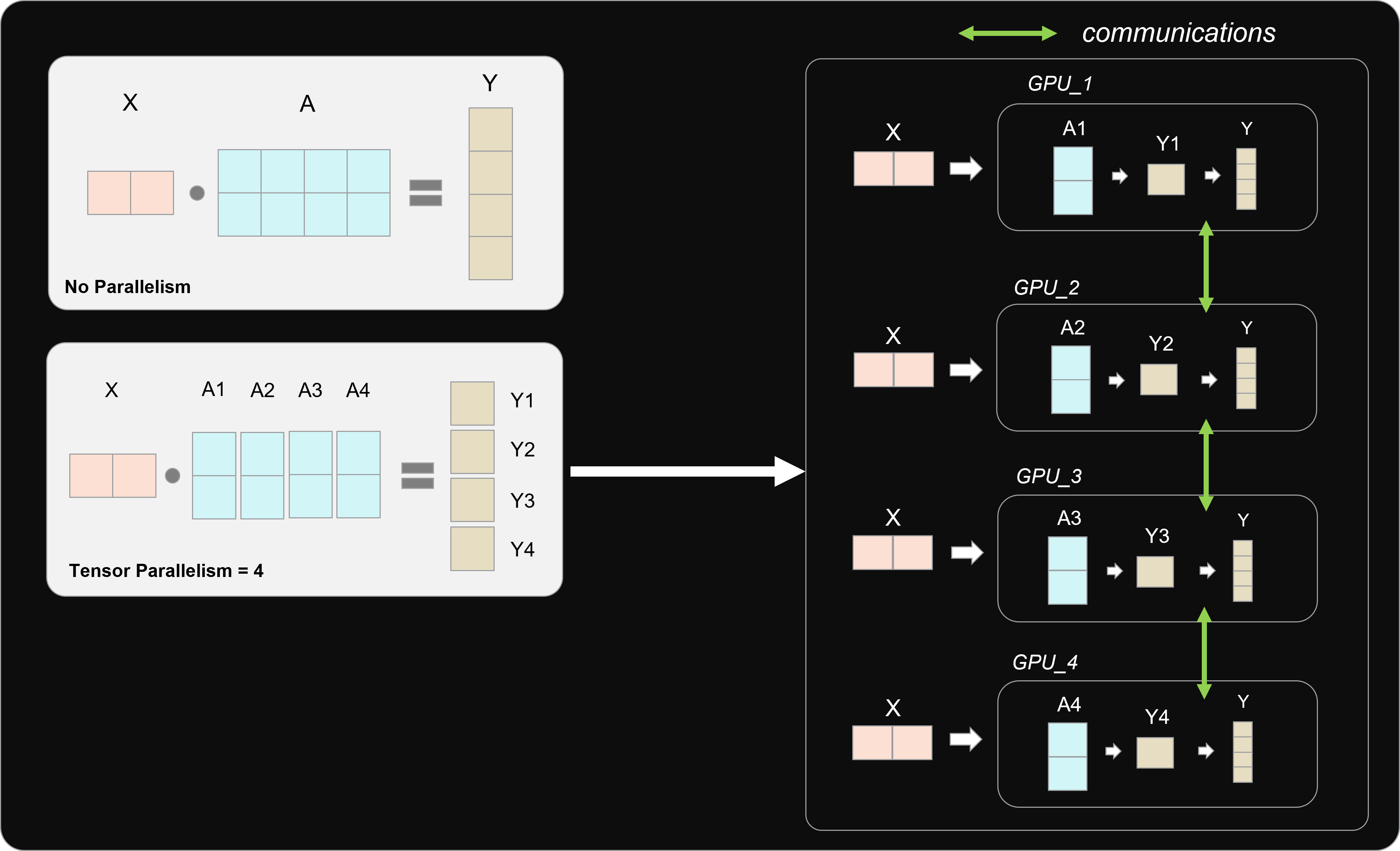
Figure 1: How Tensor Parallelism Works#
In the example above (Figure 1), the tensor labeled A is split into four parts. As part of a TP=4 configuration, each A1 through A4 is sent to its dedicated processor, yielding Y1 through Y4. After the output of this calculation has been generated for each GPU, the result is aggregated to form Y, which would be equivalent to the output for the non-parallel approach. The aggregation process involves collective communications which add a networking overhead to the process. Later in the blog, we will explore the impact of this networking overhead.
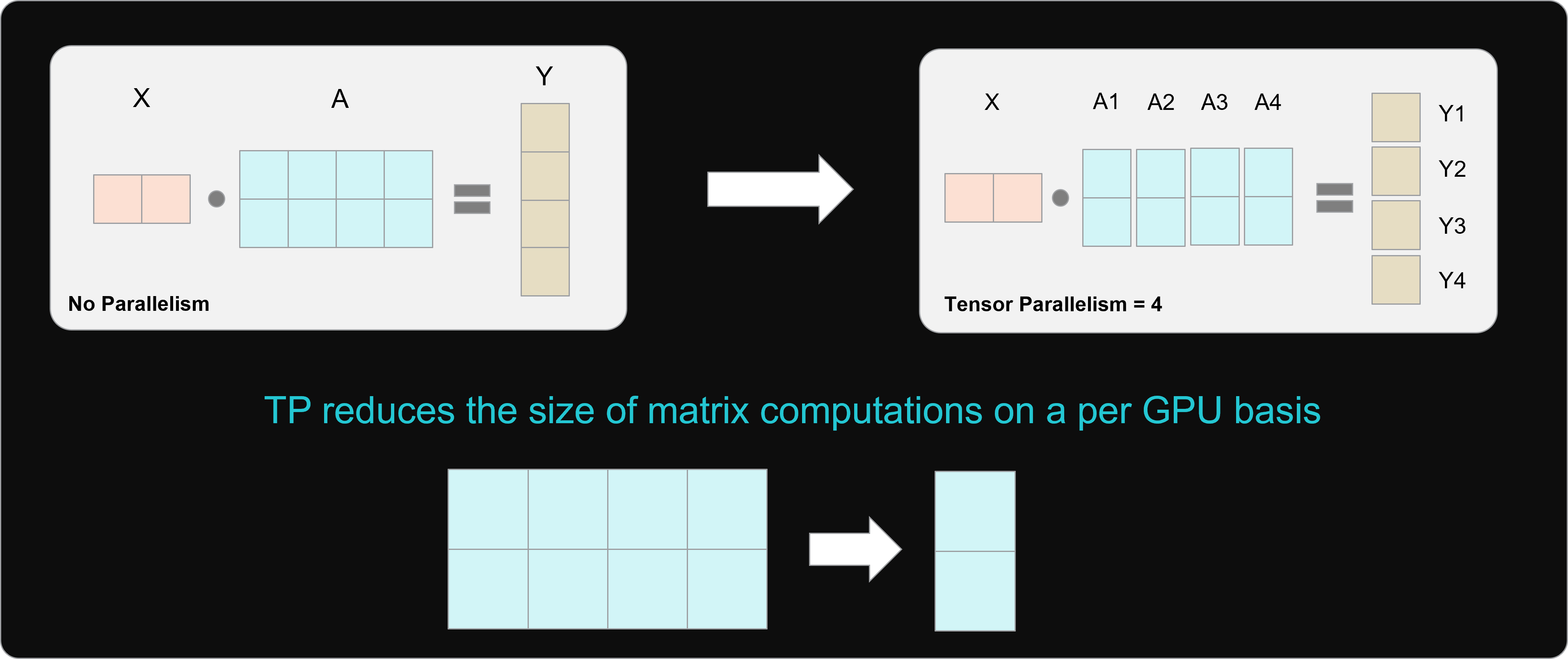
Figure 2: How Tensor Parallelism Impacts the size of matrix computations#
The image above (Figure 2) illustrates another impact of TP: the reduction in matrix sizes resulting from splitting up the tensors across GPUs. Modern GPUs are optimized to compute large matrices, but when higher TP values result in smaller matrix computations, the full computing power of the processor might be underutilized. This tends to be when small language models are deployed using TP on large data center GPUs like AMD Instinct. For these use-cases, avoiding parallelism might be more appropriate.
Tensor Parallelism Impact on Networking Overhead#
At the risk of stating the obvious, when using TP=1, no parallelism is involved, and all of the computation takes place on a single GPU. This configuration, particularly for state of the art (SoTA) LLMs like Llama 70B, has become relatively uncommon due to the memory limitations in some of the most widely used processors on the market. AMD Instinct MI300X and MI325X GPUs make deploying SoTA LLMs on a single GPU possible, reducing the need to make special considerations for networking overhead.
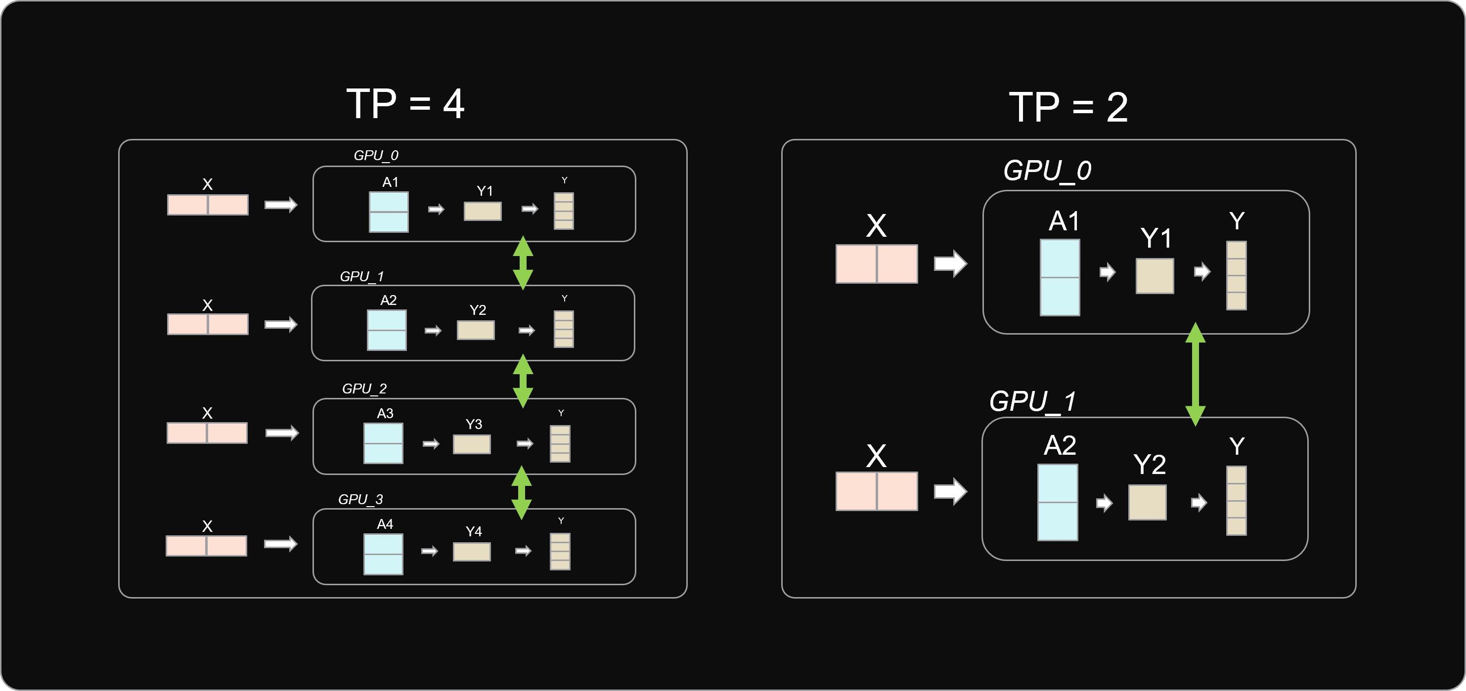
Figure 3: Tensor Parallelism settings at TP=2 vs TP=4#
For larger models, like Llama 3.1 405B and DeepSeek-R1 (671B), larger TP configurations of TP=8 are required to achieve acceptable end-to-end (E2E) latencies and throughput. However, for mid-range models like Mixtral 8x22B and Llama 3.1 70B, it might be of interest to explore TP configurations like TP=2 and TP=4:
Tensor Parallelism = 2: With two GPUs, all tensor slice exchanges, synchronization, and data transfers depend entirely on a single peer-to-peer (P2P) link. While TP=2 is feasible and not inherently risky, its impact on E2E latency can be significant for larger models. As a result, this configuration may be better suited for offline inference scenarios.
Tensor Parallelism = 4: With more GPUs, the system can leverage multiple simultaneous P2P links. Additionally, advanced communication patterns in the ROCm Collective Communications Library (RCCL) enable bandwidth sharing across links, reducing reliance on the performance of any single link.
Tensor Parallelism at Different Batch Sizes#
For this analysis, we will leverage the performance benchmarks, in figures 4 and 5, originally published as part of our inference best practices blog. The two figures report the total throughput vs E2E latency for Llama 3.1 70B FP8 across different batch sizes.
Going from Smaller to Larger TP Configurations#
When increasing TP configurations from 1 to 2, 4, and 8, the total accessible FLOPs typically double at each step. However, this increase in compute does not translate to perfectly linear scaling due to additional networking overhead. Batch size plays a crucial role in ensuring performance gains when adding GPUs to parallel inference workloads.
To further analyze the impact of decreasing TP configurations, we draw insights from Figure 4 and Table 1:
For both batch sizes (16 and 256), increasing TP from 1 to 2 and 2 to 4 results in moderate E2E latency improvements (32–41%) but significantly higher throughput gains (51–80%). This suggests that throughput is initially memory bandwidth-bound before becoming compute-bound. The doubling of compute power with higher TP configurations substantially benefits throughput.
When increasing TP from 4 to 8 with a batch size of 16, both latency and throughput improvements are minimal (11% and 12%, respectively), as the small batch size fails to fully utilize the additional four GPUs.
With a larger batch size of 256, scaling from TP4 to TP8 yields more substantial gains: latency improves by 36%, and throughput increases by 56%.
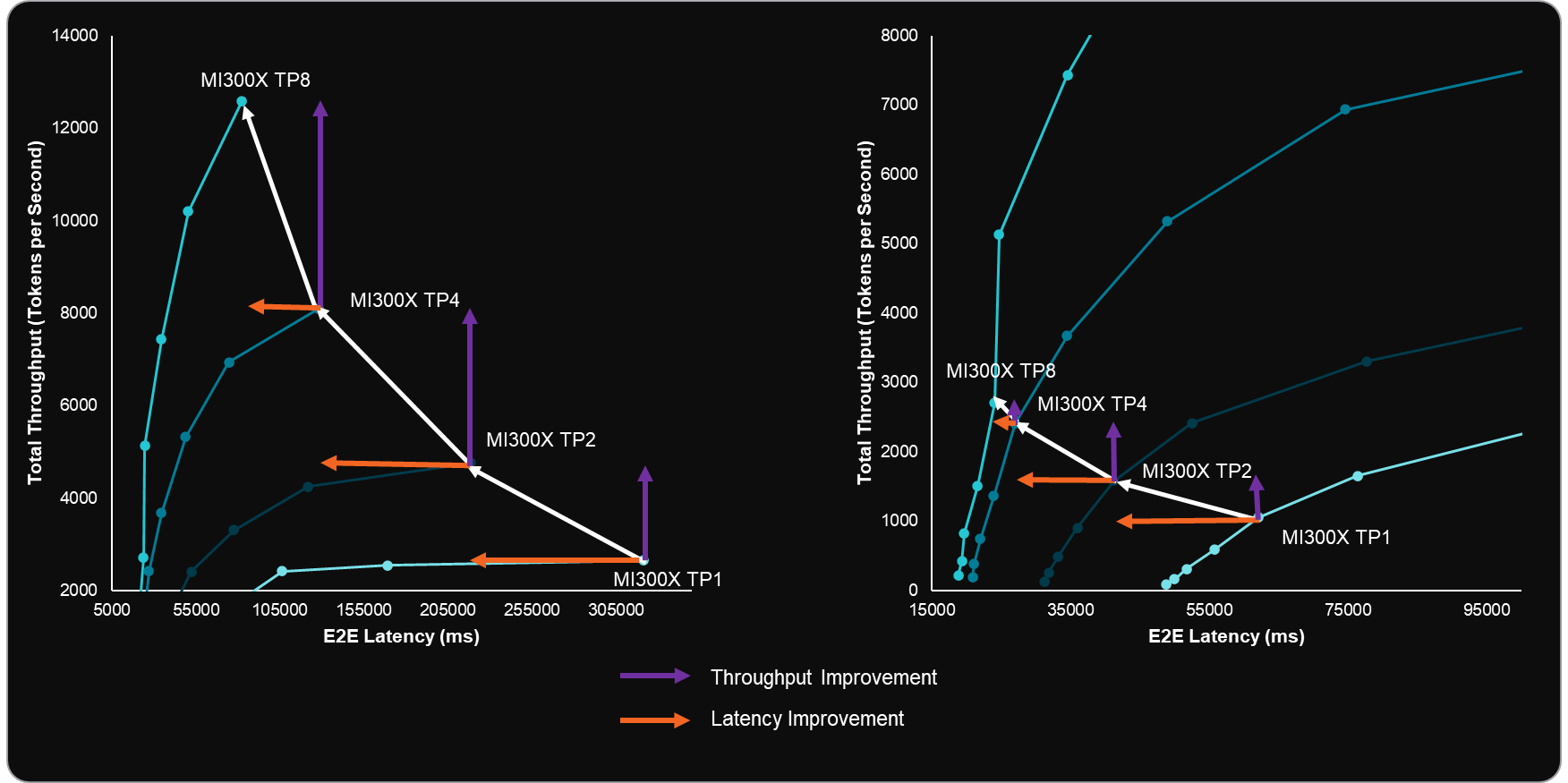
Figure 4: Llama 3.1 70B FP8 Benchmarks showing the changes in E2E latency and Total throughput across different batch size configurations. Arrows have been added to show the changes in latency and throughput as TP configurations change for batch size 256 (left) and batch size 16 (right).[1]#
Going from Larger to Smaller TP Configurations#
When transitioning from larger to smaller TP configurations, it’s essential to account for the reduction in compute power and its impact on Time to First Token (TTFT). Since prefill—the first phase of inference—is primarily compute-bound, reducing total FLOPs increases TTFT latency. One way to mitigate this is by adjusting batch size. However, scaling is not perfectly linear when moving from TP=4 to TP=2, meaning batch size does not need to be halved to maintain similar latency. Proper testing and optimization are necessary to determine the best configuration.
To further analyze the impact of decreasing TP configurations, we draw insights from Figure 5 and Table 1:
Moving from TP8 to TP4 results in only an 11–13% degradation in latency and throughput at batch size 16, presenting an opportunity to deploy two endpoints with minimal impact on user experience.
E2E latency degradation in the TP4 to TP2 transition is significantly higher at 71%. This insight is important when considering the trade-off for online inference use-cases. This likely stems from the reduction in compute capacity and the transition from 4-GPU networking to relying entirely on a single P2P interconnect.
The degradation in total throughput when scaling down from TP4 to TP2 and TP2 to TP1 is nearly linear, at 41% and 44%, respectively. For offline use cases, this provides a more stable and predictable performance decline, though careful consideration is still required.
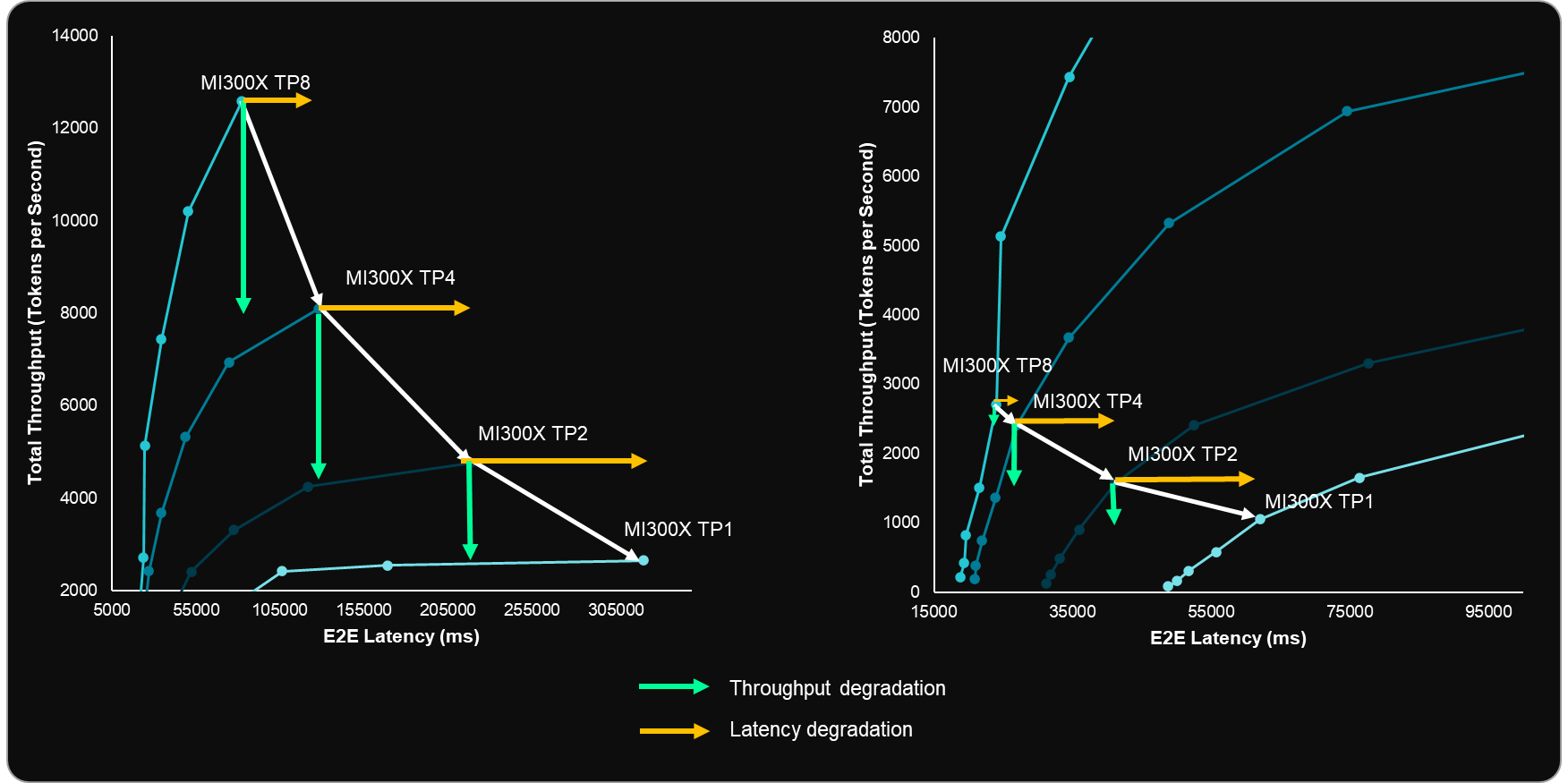
Figure 5: Llama 3.1 70B FP8 Benchmarks showing the changes in E2E latency and Total throughput across different batch size configurations. Arrows have been added to show the changes in latency and throughput as TP configurations change for batch size 256 (left) and batch size 16 (right).[1]#
Table 1, below, summarizes the percent changes when moving between TP values illustrated in figures 4 and 5. The key takeaway is that batch size is a key consideration when changing TP configurations to prevent aggressive degradation of key metrics like latency and throughput.
Metric |
Batch Size |
Increasing TP |
Decreasing TP |
||||
|---|---|---|---|---|---|---|---|
TP1→TP2 |
TP2→TP4 |
TP4→TP8 |
TP8→TP4 |
TP4→TP2 |
TP2→TP1 |
||
E2E Latency |
BS=128 |
✅ -32.0% |
✅ -41.3% |
✅ -35.0% |
❌ +54.0% |
❌ +71.0% |
❌ +47.0% |
BS=16 |
✅ -33.5% |
✅ -34.4% |
✅ -11.1% |
❌ +13.0% |
❌ +53.0% |
❌ +51.0% |
|
Total Throughput |
BS=128 |
✅ +79.6% |
✅ +70.0% |
✅ +55.5% |
❌ -36.0% |
❌ -41.0% |
❌ -44.0% |
BS=16 |
✅ +50.5% |
✅ +52.6% |
✅ +12.3% |
❌ -11.0% |
❌ -34.0% |
❌ -34.0% |
Table 1: Green checkmarks (✅) indicate improvements, while red X marks (❌) indicate degradation in performance. For E2E latency, negative percentages represent faster processing times (improvement), while for throughput, positive percentages represent higher token processing rates (improvement).
A Case for TP1 (no-parallelism)#
The use of parallelism ultimately comes down to the requirements of a specific use-case. Applications with very low latency tolerance that leverage larger models will almost always require parallelism. This is evident from the analysis in the previous section. However, there are plenty of use-cases where TP=1 will yield critical scalability, redundancy, price/performance, and enable more complex workloads.
However, memory capacity is a common limitation of going to TP=1. The figure below, aims to illustrate how the memory advantage of AMD Instinct GPUs unlocks non-parallelized deployments. Across two generations of AMD Instinct and NVIDIA GPUs, AMD GPUs retain a 1.8x-2.4x HBM memory advantage. This memory advantage enables models of up to approximately 270B parameters to be hosted on a single GPU, without the need for parallelism.
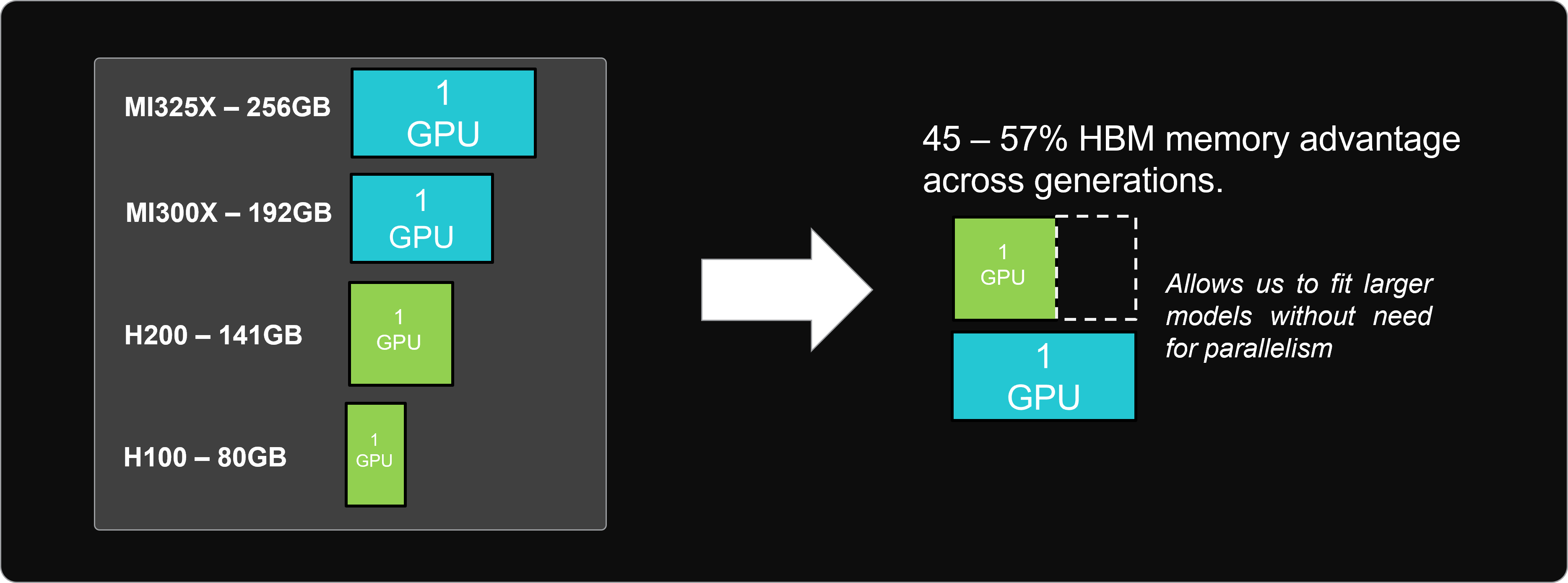
Figure 6: A comparison of per GPU HBM memory capacity for AMD Instinct MI300X, AMD Instinct MI325X, NVIDIA H100, and NVIDIA H200.[2]#
Let’s explore the benefits that this memory advantage unlocks. The figure below highlights four key opportunities unlocked by TP=1 configurations.
Scalability: Deploy multiple instances of models onto a single node to load balance traffic to multiple endpoints. This enables a greater degree of scale.
Redundancy: Multiple deployments also introduce a separation of concerns, which is crucial for microservice-based AI model deployments. If a specific service fails on a single GPU, the remaining seven GPUs can compensate, ensuring service continuity and preventing service level agreements (SLA) violations or service denial errors.
Offline Price/Performance: Deploying multiple models on a single node—where throughput is not latency-constrained—can maximize processor utilization, ensuring continuous workload execution. This approach enhances price/performance efficiency by optimizing cost per token generated.
Complex Workloads: Deploying a single model per GPU allows other processors on the node to host additional models. This is particularly beneficial for RAG and agentic applications, which rely on multiple models running in parallel or sequentially within a pipeline.
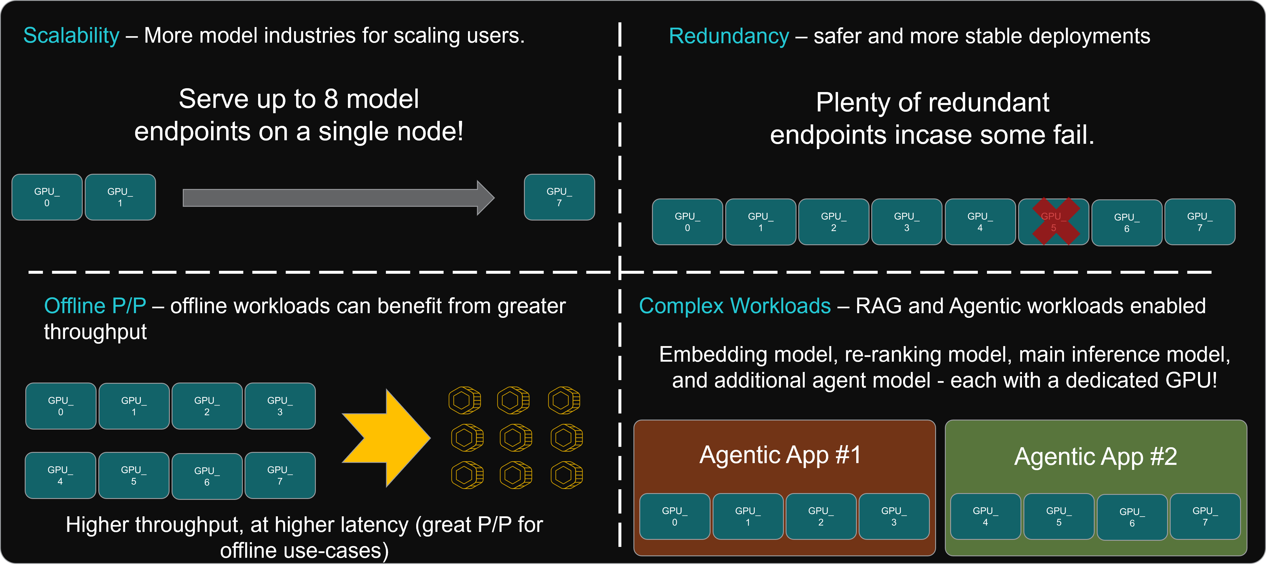
Figure 7: Analysis of benefits and opportunities of using TP=1 configurations.#
Ultimately, non-parallelism makes the most sense when the remaining processors are fully utilized to fulfill the needs of other components of an application or used to deploy multiple instances of a model on the node.
Llama 3.1 70B Multi-Model Hosting Analysis at TP1#
In many real-world applications, multiple model instances must be hosted on a single node. However, multi-model hosting introduces resource contention, especially when concurrent processes heavily utilize CPU, memory, and compute capacity. Resource allocation must be tailored to model size and workload demands to maximize efficiency, necessitating careful testing and optimization.
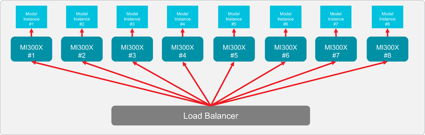
Figure 8: Simplified solution architecture, depicting a load balancer distributing requests to a single node with 8 Instinct MI300X GPUs and one model endpoint hosted per GPU.#
Multi-model hosting can be implemented using either containerized deployments with dedicated GPUs or virtual machines. The diagram above illustrates a non-parallelized (TP1) configuration on a single MI300X node, demonstrating how eight instances of the model can be distributed—one per GPU. A load balancer is typically employed to efficiently distribute application request loads across these endpoints.
When TP values are below 8 on a node with 8 GPUs, and some or all the remaining GPUs are idle, the configuration will fail to fully utilize all available compute, leading to suboptimal GPU economics. For instance, in a TP1 setup where only a single model instance is hosted, our analysis shows a 2.5× degradation in price-performance compared to TP8. While this is expected, it highlights the inefficiencies of underutilizing GPU resources.
However, significant performance gains emerge when exploring sub-TP8 configurations with multi-model hosting, leveraging the Instinct MI300X GPU’s high-bandwidth HBM3 memory. By carefully balancing model distribution across GPUs, it is possible to enhance price-performance while maintaining throughput efficiency.
The figure below highlights the price-performance impact of multi-model hosting. Key insights include:
The cost per 1M output tokens in multi-model hosting is a fraction of the TP8 scenario.
Specifically, at sub-TP8 configurations, 1M output tokens cost only 31% of the TP8 scenario, resulting in a ~69% cost savings—a direct margin benefit for businesses.
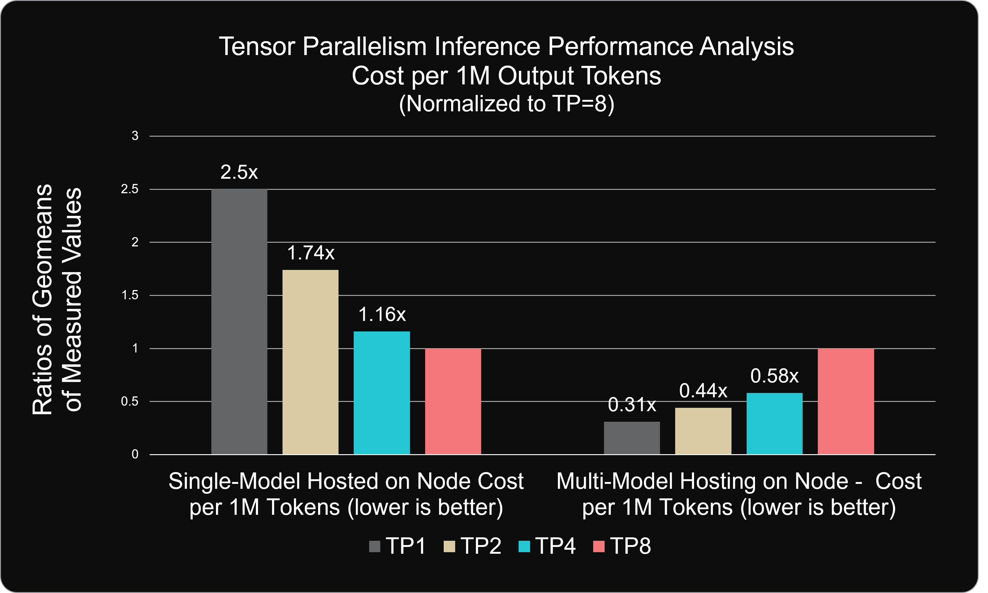
Figure 9: Analysis of costs to generate 1M output tokens normalized to the cost to generate 1M output tokens with a TP=8 configuration. The chart compares scenarios with a single model hosted at TP=1 with the remaining GPUs idle (left) and scenarios where the remaining GPUs on the node are fully utilized by additional deployments of the model (right)#
These savings are driven by a 3.21x increase in output token throughput, as eight model instances concurrently serve requests. However, this improvement comes with a notable latency trade-off. End-to-end latency increases by 2.5x compared to TP8. As a result, careful consideration must be given to the application’s latency tolerance. Workloads that can accommodate higher latency will benefit from the substantial cost reductions and throughput gains.
Summary#
This blog has provided a deep dive into how tensor parallelism (TP) configurations impact LLM inference performance, highlighting key trade-offs between networking overhead, compute efficiency, and scalability. Whether optimizing for latency-sensitive applications or cost-effective multi-model hosting, selecting the right TP configuration is crucial for balancing performance and infrastructure costs.
By reading this analysis, AI developers and solutions architects should now have a clearer understanding of how different TP settings affect throughput, latency, and total cost of ownership (TCO). More importantly, this discussion underscores that there is no universally optimal TP setting—rather, the best configuration depends on workload demands and hardware capabilities.
Looking ahead, future research and blog posts could explore additional factors influencing LLM inference efficiency, such as pipeline parallelism, mixed precision techniques, and model quantization. Additionally, an in-depth comparison of TP strategies across different GPU architectures could provide further insights for those deploying LLMs at scale.
Endnotes: