Optimizing MI300X Inter-Chiplet Communication via the RCCL Tuner API

Optimizing MI300X Inter-Chiplet Communication via the RCCL Tuner API#

June 30, 2026 by Kaiping Lu, Chunhung Wang, Kerwin Tsai, Clement Lin.

13 min read. | 3287 total words.

Performance

Developers

The AMD Instinct MI300X’s chiplet architecture introduces non-uniform communication paths when running in CPX/NPS4 mode — and RCCL default algorithms don’t account for this topology.

In this blog, you will learn how the MI300X’s XCD, IOD, and HBM hierarchy creates cross-IOD latency and bandwidth bottlenecks, how to use the RCCL Tuner Plugin API to build a rule-based, topology-aware tuner that selects the optimal algorithm and protocol per collective operation, and how to validate the results with rccl-tests.

By the end, you will have a working CSV-driven tuner plugin that automatically detects CPX/SPX mode and adapts its strategy accordingly.

Prerequisites#

Before diving in, make sure you have the following background and tools ready:

Hardware: Access to an AMD Instinct MI300X system (single-node with 8 GPUs)
Software: ROCm 6.3 or later installed, MPI runtime (e.g., OpenMPI)
Tools: amd-smi for partition mode management, rccl-tests for benchmarking
Knowledge: Familiarity with collective communication operations (AllReduce, AllGather), basic understanding of NUMA concepts, and ability to read C code

If you haven’t built RCCL from source before, refer to the RCCL GitHub repository for build instructions. The tuner plugin example is located at ext-tuner/example/ within the RCCL source tree.

Hardware Architecture: MI300X Chiplet and Non-Uniform Topology#

Before you can optimize communication on the MI300X, you need to understand its internal topology. Let’s walk through the building blocks step by step.

Building Blocks: XCD, IOD, CPX, and NPS#

The MI300X is not a monolithic chip — it is a chiplet-based design composed of multiple smaller dies connected through advanced 3D stacking. Take a look at the architecture diagram below (Source: AMD CDNA 3 architecture white paper):

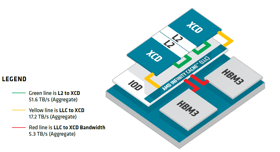
MI300X chiplet architecture showing XCD, IOD, and HBM hierarchy

Notice the three-tier bandwidth hierarchy. Each tier represents a significant bandwidth drop:

Tier	Component	Aggregate Bandwidth	What it means for you
Top	XCD (with L2 cache)	51.6 TB/s (L2 ↔ XCD)	Fastest tier — data stays within the compute die
Middle	IOD (with AMD Infinity Cache™ / LLC)	17.2 TB/s (LLC ↔ XCD)	~3x slower — data crosses from compute to I/O die
Bottom	HBM3 memory stacks	5.3 TB/s (HBM ↔ LLC)	~10x slower than top — the memory bandwidth bottleneck

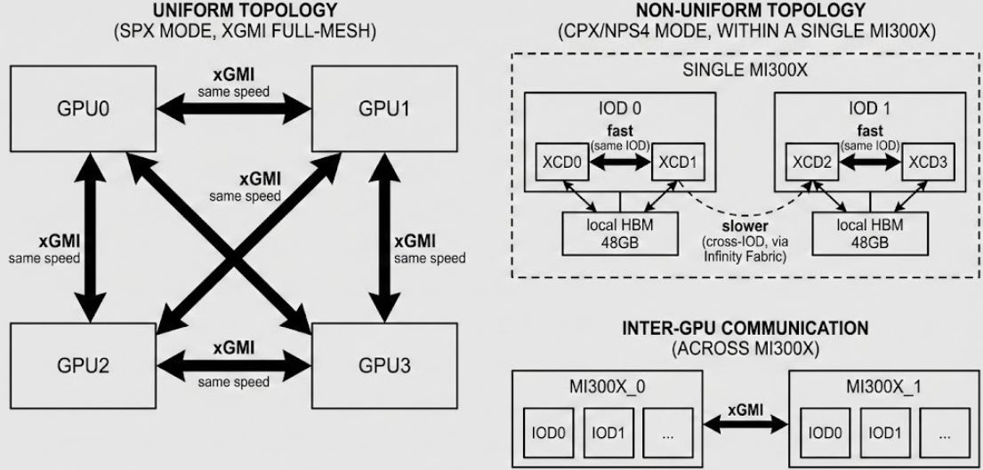
Within the same IOD, the data path follows XCD → L2 → LLC → HBM3 — fast and direct. But what happens when an XCD needs data from a different IOD? It must additionally traverse the Infinity Fabric die-to-die interconnect. Keep this in mind — it becomes critical in the next section.

Here are the key components you should know:

XCD (Accelerator Complex Die) — Each XCD contains 38 Compute Units (CUs) and its own L2 cache. The MI300X has 8 XCDs in total (304 CUs). Think of each XCD as a self-contained “mini-GPU.”

IOD (I/O Die) — Each IOD serves as the interconnect hub and memory controller, and contains the AMD Infinity Cache™ (LLC). The MI300X has 4 IODs, each managing 2 XCDs (3D-stacked on top) and 2 HBM3 stacks.

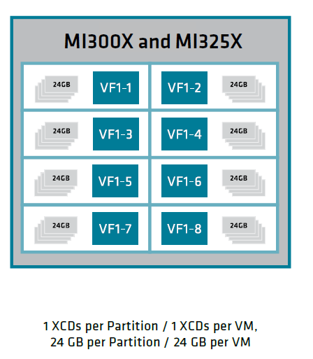
CPX (Core Partitioned Accelerator) — A compute partitioning mode that exposes each XCD as an independent logical GPU. Run amd-smi set --gpu all --compute-partition CPX to enable it.

Mode	XCDs per Logical GPU	Logical GPUs per MI300X
SPX	8	1
DPX	4	2
CPX	1	8

NPS (NUMA Per Socket) — Controls how 192 GB of HBM3 is logically divided:

	SPX (MI300X)	CPX (MI300X)
NPS1	✔	✔
NPS4		✔

In NPS1, all HBM stacks are interleaved into a single address space — software sees uniform memory. In NPS4, each IOD owns its local 48 GB. This is where things get interesting.

To check your current partition mode, run amd-smi static --partition. To switch to CPX/NPS4, use: amd-smi set --gpu all --compute-partition CPX followed by amd-smi set --gpu all --memory-partition NPS4.

Hidden Costs Beneath the Unified Memory View#

Now that you understand the building blocks, let’s examine what happens when the MI300X operates in CPX/NPS4 mode. The unified memory view from NPS1 hides several costs that become exposed — and they directly impact collective communication performance.

Cross-IOD bandwidth bottleneck — When an XCD accesses data on a different IOD, traffic must traverse the Infinity Fabric die-to-die interconnect. This bandwidth is far below local HBM access. When multiple XCDs simultaneously issue cross-IOD requests, the interconnect becomes a shared bottleneck.

Cross-IOD latency overhead — Cross-IOD access adds hop latency. Transfers between diagonally opposite IODs require two hops, further increasing latency and consuming forwarding bandwidth on intermediate IODs.

Local vs. remote access diverges under NPS4:

Local access: XCD → L2 → LLC → HBM (same IOD) — fast, no cross-die overhead
Remote access: XCD → L2 → LLC → Infinity Fabric → remote IOD → remote HBM — constrained bandwidth, higher latency

In CPX mode, each XCD becomes an independent logical GPU with a dedicated 24 GB of HBM:

MI300X CPX mode partition layout showing 8 logical GPUs

As shown, the MI300X in CPX mode is divided into 8 independent partitions (VF1-1 through VF1-8). When RCCL performs a collective like AllReduce, data transfers frequently cross IOD boundaries — and RCCL default strategy doesn’t know which ranks share an IOD and which don’t.

In CPX mode, inter-GPU communication via xGMI follows the path: local XCD → local IOD → xGMI → remote IOD → remote XCD. This compounds both intra-chip cross-IOD and inter-chip xGMI costs. Every logical GPU communication potentially involves two levels of non-uniform overhead.

From Uniform to Non-Uniform: The Case for a Tuner#

So why can’t RCCL handle this automatically? As described in “Hidden Costs Beneath the Unified Memory View”, RCCL default tuning model assumes:

All GPU-to-memory paths have uniform latency and bandwidth
Algorithms (Ring vs. Tree) and protocols (Simple, LL, LL128) are selected based on a generic model
No distinction between same-IOD and cross-IOD communication costs

Under xGMI full-mesh topology (SPX mode), this works fine — all GPU-to-GPU paths are roughly similar. But in CPX/NPS4 mode, the paths are no longer uniform:

Non-uniform communication paths in CPX/NPS4 mode

A custom tuner plugin can make topology-aware decisions at runtime. Here’s what it enables:

Decision Point	Default Behavior	What the Tuner Does
Algorithm selection	Generic model, path-unaware	Selects Tree or Ring based on topology and message size
Protocol selection	Based on message size only	Chooses LL, LL128, or Simple considering path characteristics
Channel count	Fixed or heuristic	Adjusts channels based on actual interconnect bandwidth
Config switching	Static configuration	Detects CPX/SPX mode at `init()`, loads the right config file

The key insight: the optimal communication strategy depends on both the message size AND the physical topology of the data path.

RCCL Tuner API Deep Dive#

Now that you understand why a tuner is needed, let’s explore how the RCCL Tuner Plugin API works. This section covers the API structure, the rule-based decision flow, and why a plugin is superior to environment variables.

API Structure: `ncclTuner_v5_t`#

The RCCL Tuner plugin is a shared library (.so file) that RCCL loads at runtime. It must export a symbol ncclTunerPlugin_v5 of type ncclTuner_v5_t:

typedef struct {
  const char* name;

  ncclResult_t (*init)(
    void** context, uint64_t commId,
    size_t nRanks, size_t nNodes,
    ncclDebugLogger_t logFunction,
    ncclNvlDomainInfo_v5_t* nvlDomainInfo,
    ncclTunerConstants_v5_t* constants
  );

  ncclResult_t (*getCollInfo)(
    void* context, ncclFunc_t collType,
    size_t nBytes, int numPipeOps,
    float** collCostTable, int numAlgo, int numProto,
    int regBuff, int* nChannels
  );

  ncclResult_t (*finalize)(void* context);
} ncclTuner_v5_t;

The lifecycle is straightforward — three functions, called at three points:

init() — Called once when ncclCommInitRank() creates a communicator. Read topology info, load your config files, and allocate state here.
getCollInfo() — Called for every collective operation. This is where you influence algorithm/protocol selection.
finalize() — Called on ncclCommFinalize(). Clean up your resources.

Rule-Based Decision: How `getCollInfo` Works#

In our implementation, we don’t manually tune the internal cost table. Instead, we define declarative rules in a CSV config file and let getCollInfo match the current collective against these rules at runtime.

Each time RCCL is about to execute a collective, it calls getCollInfo() with the following runtime context:

Runtime Context	What it tells you
`collType`	What operation? (AllReduce, AllGather, …)
`nBytes`	How large is the message?
`nRanks` / `nNodes`	How many ranks and nodes?
`numPipeOps`	How many pipelined operations?

The plugin iterates through its loaded rules and applies the first match. Here’s the format:

Rule Format:
  colltype, minbytes, maxbytes, algorithm, protocol, channels, nNodes, nRanks

Example:
  allreduce, 0, 262144, tree, ll, -1, 1, 64

Matching Logic:
  if (rule.collType == collType &&
      nBytes >= rule.minBytes && nBytes <= rule.maxBytes &&
      rule.nNodes == nNodes && rule.nRanks == nRanks)
    → apply this rule

Here’s what each field does:

Rule Field	Meaning
`colltype`	Which collective to match (`allreduce`, `allgather`, `reducescatter`, …)
`minbytes` / `maxbytes`	Message size range this rule applies to
`algorithm`	`tree` or `ring`
`protocol`	`ll` (Low-Latency), `ll128`, or `simple`
`channels`	Number of channels (`-1` = let RCCL decide)
`nNodes` / `nRanks`	Topology filter — only apply when topology matches

Why rules instead of manual cost table tuning? The underlying API uses a cost table (collCostTable[algo][proto]), but directly manipulating cost values requires deep knowledge of RCCL internal latency model. The rule-based approach abstracts this: when a rule matches, the plugin sets the preferred algo/proto cost to 0.0 (lowest cost wins). You focus on what to select, not how the cost model works.

If no rule matches, getCollInfo() returns without modifying anything and RCCL falls back to its default tuning. This means your plugin never makes things worse for uncovered scenarios — a safe design pattern.

Plugin vs. Environment Variables#

You might ask: “Can’t I just set NCCL_ALGO=RING and NCCL_PROTO=SIMPLE as environment variables?” Yes — but that’s a static, global decision. Compare the two approaches:

Aspect	Environment Variables	Tuner Plugin
Granularity	One setting for ALL collectives	Per-collective, per-size
Adaptability	Fixed at process start	Runtime topology-aware
Message size awareness	✗	✔
Collective type awareness	✗	✔
Topology awareness	✗	✔
Fallback safety	If wrong, everything suffers	RCCL falls back to defaults

Consider this scenario: for a 1 KB AllReduce (latency-bound), you want Tree + LL. For a 1 GB AllReduce (bandwidth-bound), you want Ring + Simple. A tuner handles both cases with different rules; a single environment variable cannot.

Implementation: A CPX-Aware Tuner Plugin#

Ready to build your own tuner? This section walks you through the RCCL example plugin, shows you how to extend it for CPX-awareness, and gets it running on your system.

Code Walkthrough: CSV-Driven Plugin#

The RCCL repository includes an example tuner plugin that reads tuning configurations from a CSV file. Let’s walk through the key components.

Step 1: Define the plugin entry point#

Every RCCL tuner plugin must export a ncclTunerPlugin_v5 symbol. This tells RCCL which functions to call:

const ncclTuner_v5_t ncclTunerPlugin_v5 = {
  .name      = "Example",
  .init      = pluginInit,
  .getCollInfo = pluginGetCollInfo,
  .finalize  = pluginFinalize
};

Step 2: Initialize and load rules#

In pluginInit(), allocate your context and load tuning rules from a config file:

ncclResult_t pluginInit(void** context, uint64_t commId,
                        size_t nRanks, size_t nNodes,
                        ncclDebugLogger_t logFunction,
                        ncclNvlDomainInfo_v5_t* nvlDomainInfo,
                        ncclTunerConstants_v5_t* constants) {
  TunerContext* ctx = (TunerContext*)malloc(sizeof(TunerContext));
  ctx->nRanks = nRanks;
  ctx->nNodes = nNodes;
  ctx->logFunction = logFunction;

  const char* configFile = getenv("NCCL_TUNER_CONFIG_FILE");
  if (!configFile) configFile = "nccl_tuner.conf";
  loadConfig(ctx, configFile);

  *context = ctx;
  return ncclSuccess;
}

Step 3: Match rules in `getCollInfo()`**#

For each collective call, iterate through loaded rules and apply the first match:

ncclResult_t pluginGetCollInfo(void* context, ncclFunc_t collType,
                               size_t nBytes, int numPipeOps,
                               float** collCostTable,
                               int numAlgo, int numProto,
                               int regBuff, int* nChannels) {
  TunerContext* ctx = (TunerContext*)context;
  float (*table)[NCCL_NUM_PROTOCOLS] =
    (float (*)[NCCL_NUM_PROTOCOLS])collCostTable;

  for (int i = 0; i < ctx->numConfigs; i++) {
    TuningConfig* config = &ctx->configs[i];
    if (config->collType == collType &&
        nBytes >= config->minBytes &&
        nBytes <= config->maxBytes &&
        /* topology matching ... */) {
      table[config->algorithm][config->protocol] = 0.0;
      if (config->nChannels != -1)
        *nChannels = config->nChannels;
      return ncclSuccess;
    }
  }
  return ncclSuccess;
}

Step 4: Write your config file**#

Create nccl_tuner_nps4.conf with your tuning rules:

# colltype, minbytes, maxbytes, algorithm, protocol, channels, nNodes, nRanks
allreduce, 0, 262144, tree, ll, -1, 1, 64

This rule tells the plugin: for AllReduce with messages ≤ 256 KB on a single-node 64-rank setup, use Tree + LL.

Why does Tree + LL work well here? In CPX/NPS4 mode with 64 ranks, a Ring AllReduce requires 2(n-1) = 126 sequential steps, each traversing cross-IOD and cross-GPU links. A Tree AllReduce requires only 2·log₂(n) = 12 steps — a 10x reduction. Combined with the LL protocol’s lower per-message latency, Tree + LL significantly reduces end-to-end latency for small, latency-bound messages.

Tree + LL advantage reverses for large messages. Tree’s fan-in/fan-out creates bandwidth bottlenecks at root nodes, and LL 50% data overhead becomes significant. Always bound your Tree + LL rules to small message sizes and add separate ring, simple rules for larger transfers.

Step 5: Add CPX/SPX auto-detection#

To make the plugin topology-aware, read the Linux sysfs to detect the current compute partition mode:

static int detect_cpx_mode(void) {
    for (int card = 0; card < 16; card++) {
        char path[256];
        char buf[64] = {0};

        snprintf(path, sizeof(path),
                 "/sys/class/drm/card%d/device/current_compute_partition", card);

        FILE* f = fopen(path, "r");
        if (!f) continue;

        if (fgets(buf, sizeof(buf), f)) {
            buf[strcspn(buf, "\n")] = 0;
            fclose(f);
            if (strcmp(buf, "CPX") == 0) return 1;
            if (strcmp(buf, "SPX") == 0) return 0;
            return -1;
        }
        fclose(f);
    }
    return -1;
}

Then use it in pluginInit() to load the right config file:

ncclResult_t pluginInit(void** context, ...) {
    TunerContext* ctx = (TunerContext*)malloc(sizeof(TunerContext));
    // ... initialize ctx ...

    int isCpxMode = detect_cpx_mode();
    if (isCpxMode == 1) {
        loadConfig(ctx, "/path/to/nccl_tuner_nps4.conf");
    } else {
        loadConfig(ctx, "/path/to/nccl_tuner_nps1.conf");
    }

    *context = ctx;
    return ncclSuccess;
}

The plugin now automatically adapts:

CPX mode → Loads NPS4-specific rules optimized for cross-IOD NUMA topology
SPX mode → Loads NPS1 rules using default strategies for unified memory

Try verifying the detection by running with NCCL_DEBUG=INFO NCCL_DEBUG_SUBSYS=TUNING — the plugin should log which config file it loaded.

Build and Install#

Follow these steps to build and deploy your tuner plugin:

Step 1: Build the plugin#

cd $RCCL_HOME/ext-tuner/example/
make

This produces libnccl-tuner.so.

Step 2: Set environment variables and run**#

export NCCL_TUNER_PLUGIN=/path/to/libnccl-tuner.so
export NCCL_DEBUG=INFO
export NCCL_DEBUG_SUBSYS=TUNING

The plugin auto-detects CPX/SPX mode at initialization — no need to manually specify NCCL_TUNER_CONFIG_FILE.

Common pitfall: If the plugin doesn’t load, verify the .so file path is correct and the file has read permissions. Check the RCCL debug output for messages like TUNER: Initializing tuner.... If you see no tuner-related messages, the path is likely wrong.

Performance Validation#

With your tuner plugin built and configured, let’s validate it. This section shows you how to run benchmarks and interpret the results.

Benchmark Setup#

Use the rccl-tests suite to benchmark AllReduce on an 8x MI300X node in CPX/NPS4 mode (64 ranks).

Test environment: Single node with 8 AMD Instinct MI300X GPUs, CPX compute partition, NPS4 memory partition (64 logical GPUs), ROCm 7.2, RCCL develop branch, OpenMPI 5.0.

Step 1: Run baseline (default RCCL — typically Ring + Simple)#

mpirun -np 64 --bind-to numa \
  rccl-tests/build/all_reduce_perf -b 1 -e 128M -f 2 -g 1

Step 2: Run with tuner plugin#

mpirun -np 64 --bind-to numa \
  -x NCCL_TUNER_PLUGIN=/path/to/libnccl-tuner.so \
  rccl-tests/build/all_reduce_perf -b 1 -e 128M -f 2 -g 1

Step 3 (optional): Profile all algorithm/protocol combinations#

To understand which combination works best at each message size, run all six combinations individually:

# Ring + Simple (default baseline)
mpirun -np 64 --bind-to numa -x NCCL_ALGO=ring -x NCCL_PROTO=simple \
  rccl-tests/build/all_reduce_perf -b 1 -e 128M -f 2 -g 1

# Tree + LL (optimized for small messages)
mpirun -np 64 --bind-to numa -x NCCL_ALGO=tree -x NCCL_PROTO=ll \
  rccl-tests/build/all_reduce_perf -b 1 -e 128M -f 2 -g 1

# Repeat for: ring+ll, ring+ll128, tree+ll128, tree+simple
# Note: some combinations require additional env vars or source patches.
# See "Reproducibility notes" in the results analysis section for details.

Compare the time and busbw columns across all runs to identify the optimal algorithm/protocol for each message size range.

Troubleshooting: If you see no performance difference, check:

Is the tuner actually loaded? Look for TUNER related information in the debug output.
Do your rules match the test topology? Verify nRanks and nNodes in your config match the actual run.
Is the message size range covered? Rules only apply within their minbytes-maxbytes range.

Results Analysis#

To understand the performance landscape, we benchmarked all six algorithm/protocol combinations for 64-rank AllReduce on a single MI300X node in CPX/NPS4 mode. The results reveal clear performance zones that inform tuner rule design.

Tree+LL latency speedup vs. default RCCL (Ring+Simple)#

The following figure shows the latency speedup of Tree + LL relative to the default RCCL behavior (Ring + Simple). Values above the 1.0x baseline indicate Tree + LL is faster.

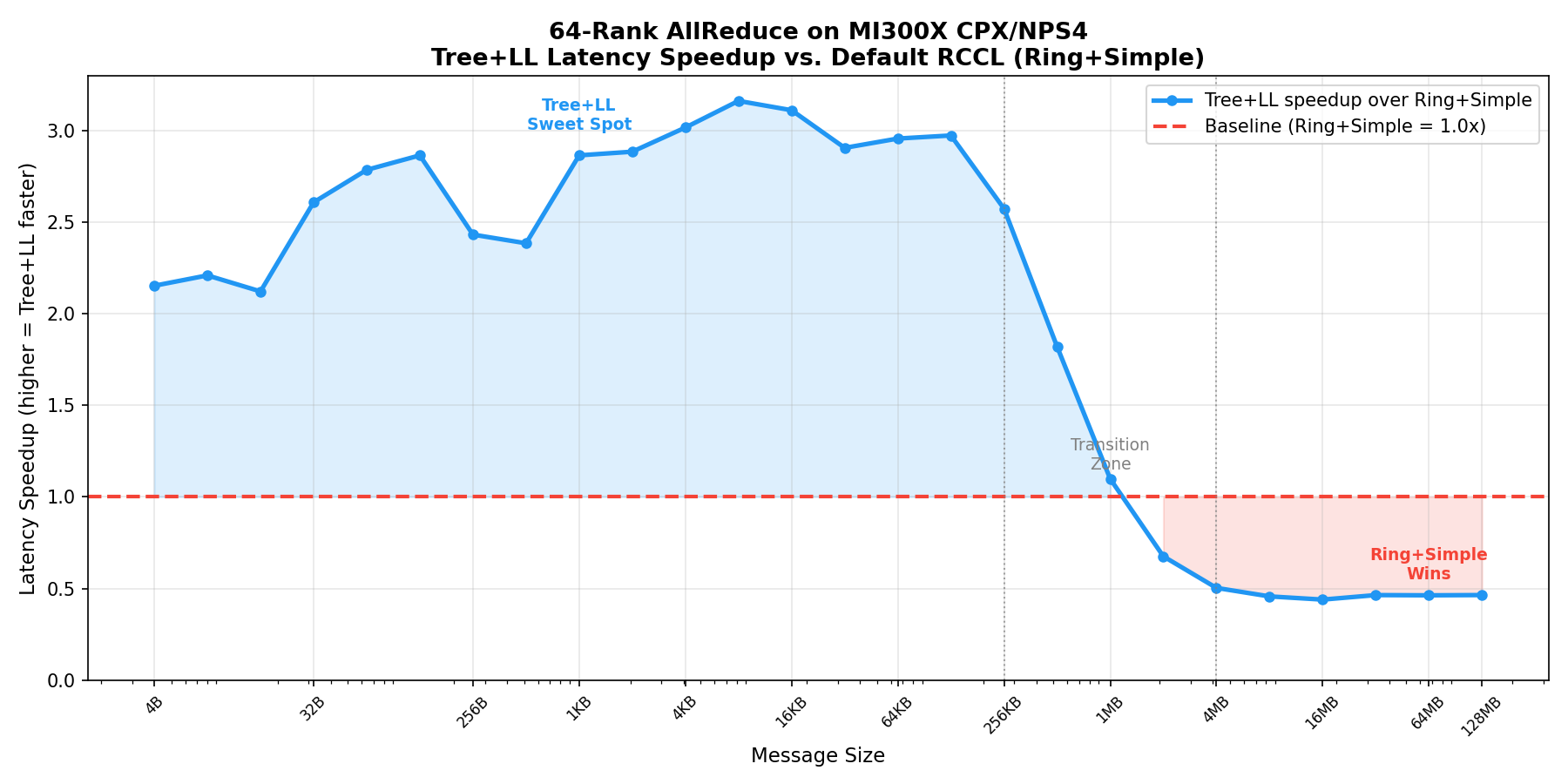
Bell curve showing Tree+LL speedup over Ring+Simple

The curve reveals that Tree + LL delivers 2-3x lower latency across a wide range of small message sizes, with peak speedup of ~3.1x around 4 KB - 16 KB. The crossover point — where Ring + Simple becomes faster — occurs around 1-4 MB.[1]

Bus bandwidth across all algorithm/protocol combinations#

The next figure compares the achieved bus bandwidth for all six combinations, showing how each configuration saturates at different throughput levels.

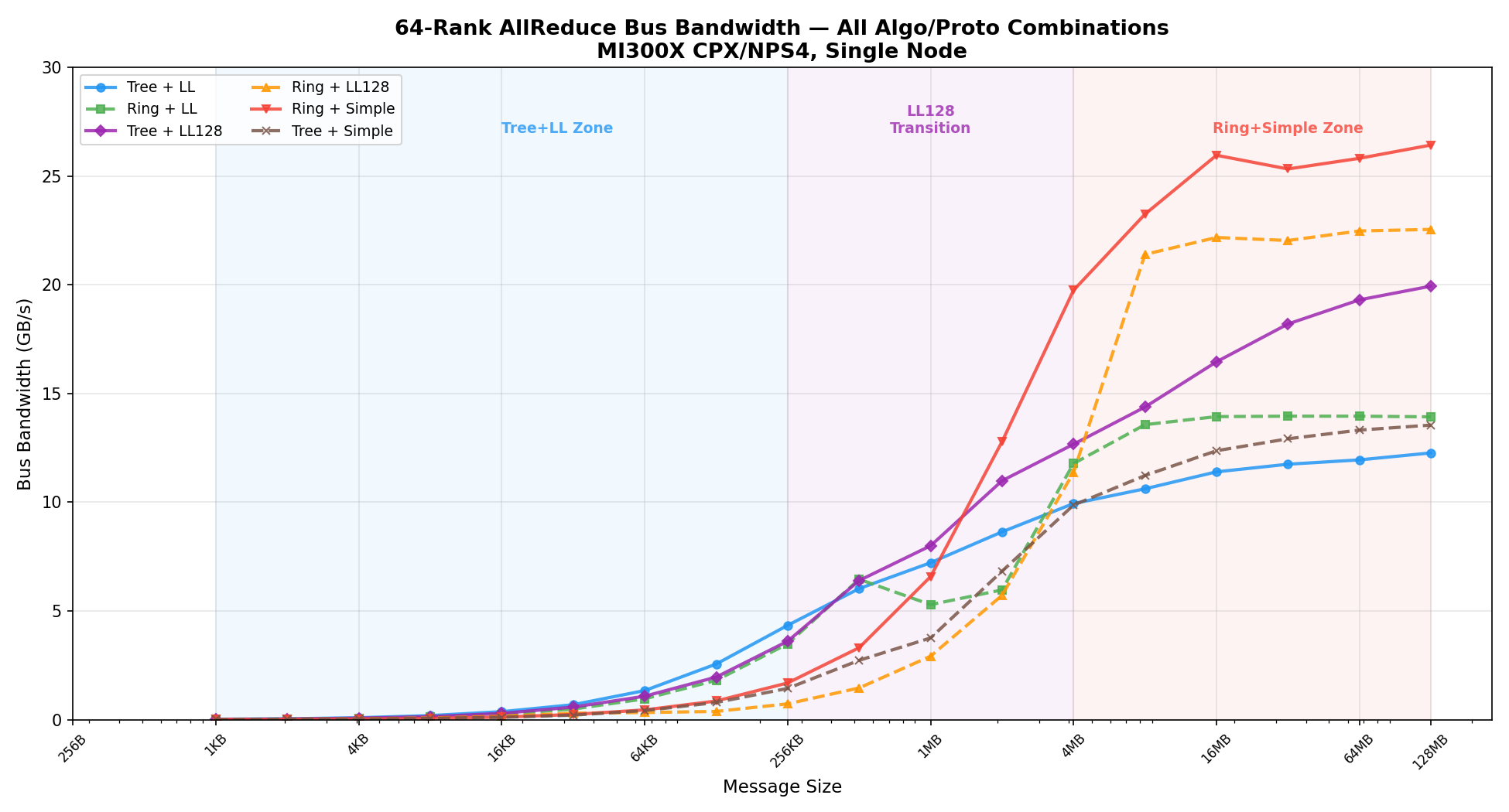
Bus bandwidth comparison across all algorithm and protocol combinations

Ring + Simple reaches the highest peak bandwidth (~26 GB/s), while Tree + LL saturates around ~12 GB/s due to the LL protocol’s 50% data overhead. Tree + LL128 offers a middle ground, reaching ~20 GB/s — making it the best choice in the transition zone.

Latency comparison (representative message sizes)#

The following table shows measured out-of-place latency (in microseconds) for each combination. The lowest latency per row is highlighted:

Size	Tree+LL	Ring+LL	Tree+LL128	Ring+LL128	Ring+Simple	Tree+Simple
32 B	76	70	106	97	198	244
1 KB	94	154	123	203	268	248
16 KB	87	129	111	197	271	302
256 KB	119	148	143	706	306	359
1 MB	286	390	258	708	314	549
4 MB	831	701	652	726	418	836
128 MB	21541	18970	13251	11720	9996	19503

Three distinct performance zones emerge from the data:

Message Size Range	Best Configuration	Why
< 256 KB	Tree + LL	Tree’s logarithmic step count (12 vs Ring’s 126) dominates; LL protocol minimizes per-step latency. Speedup: 2-3x over default.
256 KB - 4 MB	Tree + LL128	LL128 reduces data overhead compared to LL while retaining Tree’s step advantage. This transition zone bridges latency-bound and bandwidth-bound regimes.
> 4 MB	Ring + Simple	Communication becomes bandwidth-bound. Ring’s pipelined data flow and Simple protocol’s full-bandwidth transfers yield the highest throughput (~26 GB/s).

Why these zones? The latency model#

RCCL internally estimates the cost of each algorithm/protocol combination using a latency model. Understanding this model explains why the zone boundaries fall where they do.

For a given message of nBytes, the estimated time is:

time = latency + nBytes / bandwidth

Where latency depends on the algorithm’s step count:

Algorithm	Step Count (nRanks = 64)	Latency Formula
Ring	2 x nRanks - 1 = 127	baseLat + 127 x hwLat
Tree	2 x log2(nRanks) = 12	baseLat + 12 x hwLat

For small messages, nBytes / bandwidth is negligible — latency dominates. Tree’s 12-step path is ~10x fewer hops than Ring’s 127 steps, which directly translates to the 2-3x speedup we measured.

As message size grows, the nBytes / bandwidth term takes over. Tree’s fan-in/fan-out topology creates bandwidth bottlenecks at interior nodes, while Ring’s pipelined data flow achieves higher sustained throughput. This is why Ring + Simple overtakes Tree + LL around 1-4 MB.

The LL protocol adds another dimension: it uses 4-byte flags per 8-byte payload (50% overhead), limiting effective bandwidth. LL128 reduces this overhead by packing 120 useful bytes per 128-byte line (~6% overhead), explaining why Tree + LL128 outperforms Tree + LL in the transition zone.

Recommended tuner configuration#

In the implementation walkthrough, we started with a single Tree + LL rule targeting small messages. The profiling results above reveal that a complete configuration needs additional rules for the transition and bandwidth-bound zones. A production-ready config file for 64-rank CPX/NPS4 AllReduce should use three rules:

# colltype, minbytes, maxbytes, algorithm, protocol, channels, nNodes, nRanks
allreduce, 0, 262144, tree, ll, -1, 1, 64
allreduce, 262145, 4194304, tree, ll128, -1, 1, 64
allreduce, 4194305, 17179869184, ring, simple, -1, 1, 64

Reproducibility notes#

Not all algorithm/protocol combinations are available by default in RCCL on MI300X (gfx942). The following table summarizes what is needed to test each combination:

Algo + Proto	How to Enable	Additional Requirements	Reason
Ring + Simple	`NCCL_ALGO=ring NCCL_PROTO=simple`	None (default behavior)	RCCL default selection for MI300X
Ring + LL	`NCCL_ALGO=ring NCCL_PROTO=ll`	None	Supported out of the box
Tree + LL	`NCCL_ALGO=tree NCCL_PROTO=ll`	None	Supported out of the box
Ring + LL128	`NCCL_ALGO=ring NCCL_PROTO=ll128`	`RCCL_LL128_FORCE_ENABLE=1`	LL128 is disabled by default for certain topologies on MI300X
Tree + LL128	`NCCL_ALGO=tree NCCL_PROTO=ll128`	`RCCL_LL128_FORCE_ENABLE=1`	Same as above
Tree + Simple	Not available via env vars	Source code patch required	RCCL unconditionally blocks Tree+Simple on gfx942/gfx950 single-node in `ncclTopoTuneModel()` (`tuning.cc`). Setting `NCCL_ALGO=tree NCCL_PROTO=simple` is silently ignored — RCCL falls back to another combination. The data in this blog was collected using a custom patch that adds an `RCCL_PARAM(ForceTreeSimple)` override.

The tuner plugin is not subject to these restrictions when selecting Ring+LL128 or Tree+LL128, because it modifies the internal cost table directly. However, Tree+Simple cannot be selected even by the tuner — RCCL marks it as IGNORE in the cost table before the tuner runs, so setting its cost to 0.0 has no effect.

Key takeaways from the results:

The sweet spot for Tree + LL is 4 B - 256 KB: Tree’s hierarchical reduction reduces the 126-step Ring path to just 12 steps. Combined with LL low per-message latency, this yields up to 3.1x speedup over the default Ring + Simple configuration.
The crossover occurs at 1-4 MB, not 256 KB: Tree + LL remains faster than Ring + Simple well beyond 256 KB. A middle-ground configuration using Tree + LL128 bridges the gap between the latency-bound and bandwidth-bound regimes.
A three-zone config outperforms any single rule: No single algorithm/protocol combination is optimal across all message sizes. The recommended three-rule config ensures each size range uses its best-performing combination, while RCCL default tuning handles any uncovered scenarios.
Extend to other collectives: Profile your actual AI training workload to identify which collective types (AllGather, ReduceScatter) and message sizes dominate, then add corresponding rules to your config file.

Summary#

Optimized RCCL configurations can improve small message AllReduce latency and deliver balanced performance across message sizes on AMD Instinct™ MI300X GPU systems.[1]

MI300X CPX/NPS4 mode exposes a non-uniform communication topology that generic collective tuning does not fully capture. By walking through the XCD, IOD, HBM, and xGMI data paths, this blog showed why collective performance varies with message size and why a single, static algorithm choice is often too coarse for real workloads.

You also learned how to turn that topology knowledge into an actionable RCCL tuner plugin. Starting from the RCCL example plugin, you built a CSV-driven rule system, added CPX/SPX mode auto-detection through sysfs, and used rccl-tests to validate which algorithm and protocol combinations perform best across the latency-bound, transition, and bandwidth-bound message ranges. The result was a three-zone tuner configuration — Tree + LL for small messages, Tree + LL128 for the transition zone, and Ring + Simple for large transfers — that covers the full size spectrum while safely falling back to RCCL defaults for anything uncovered.

The main deliverable is a repeatable tuning workflow rather than a one-off config: profile your target collective patterns, map each message-size range to its best algorithm and protocol, encode those choices as tuner rules, and validate every change before applying it to production training. Use this approach as a starting point for adapting RCCL tuning to your own MI300X topology and application mix.

Additional Resources#

Disclaimers#

Third-party content is licensed to you directly by the third party that owns the content and is not licensed to you by AMD. ALL LINKED THIRD-PARTY CONTENT IS PROVIDED “AS IS” WITHOUT A WARRANTY OF ANY KIND. USE OF SUCH THIRD-PARTY CONTENT IS DONE AT YOUR SOLE DISCRETION AND UNDER NO CIRCUMSTANCES WILL AMD BE LIABLE TO YOU FOR ANY THIRD-PARTY CONTENT. YOU ASSUME ALL RISK AND ARE SOLELY RESPONSIBLE FOR ANY DAMAGES THAT MAY ARISE FROM YOUR USE OF THIRD-PARTY CONTENT.

[1] (1,2)

MI300-101 Testing by AMD as of March 2026, on a single-node system with 8× AMD Instinct™ MI300X GPUs configured in CPX compute partition and NPS4 memory partition (64 logical GPUs / 64 ranks). Benchmark: rccl-tests all_reduce_perf (build develop:6405c76), message sizes 1 B–128 MB; each result is the average of 20 measured iterations with 5 warmup iterations; correctness validation enabled.
For small message sizes (<256 KB), a tuner-selected Tree + LL configuration reduced AllReduce latency by approximately 2–3× versus the default Ring + Simple configuration, with peak improvement of ~3.1× for 4–16 KB messages. For larger message sizes (~1–4 MB and above), performance advantages transition, with the default Ring + Simple configuration achieving the highest bus bandwidth (~26 GB/s). Tree + LL128 provides balanced performance (~20 GB/s peak bus bandwidth) across intermediate message sizes (256 KB–4 MB).
RCCL communication algorithms and protocols are designed to optimize performance differently based on message size, with low-latency protocols favoring small transfers and bandwidth-optimized protocols favoring larger transfers.
Actual results may vary based on system configuration, software versions, and workload (MI300-101).