Exploring XGBoost: A Deep Dive

August 18, 2026 by Ish Kool, Vivek Kumar, Karthik Kashyap Thatipamula, Vikas C Sajjan, Vish Vadlamani, Phani Vaddadi.

17 min read. | 4237 total words.

Software tools & optimizations

C++, AI/ML, Scientific Computing, Linear Algebra

Data Science, AI, Developers

XGBoost (Extreme Gradient Boosting) is an open-source library that implements gradient-boosted decision trees, an ensemble method that builds an additive sequence of trees where each new tree is fit to the gradient of the loss left by the ones before it. It supports regression, classification, ranking, and survival objectives behind a single training loop, and is implemented as a high-performance C++ core with CPU and CUDA/HIP backends, exposed through Python, R, and JVM bindings. On large tabular datasets it is a standard production choice for both accuracy and training throughput. This blog opens the box on how it works, end to end.

Part 1 rebuilds the math from scratch — what gradient boosting is, why second-order Newton boosting drops out naturally, how a single algorithm absorbs regression, classification, ranking, and survival analysis through a swap of objective function, and how the regularization term keeps trees honest.

Part 2 then walks the actual XGBoost source tree: the module map, where training and prediction live, the parameters that shape every tree, the CPU vs. GPU split, the kernels that drive tree_method="hist" on AMD Instinct GPUs, the data layouts (DMatrix, QuantileDMatrix, EllpackPage) that make all of it fast, a hand-worked example tree, and a closing tour of published benchmarks. By the end you should be able to read a stack trace from Learner::UpdateOneIter down to a StHistKernel dispatch and know exactly what each layer is doing — and why.

---

Part 1 — The Math: From a Single Tree to Gradient Boosting

Decision Trees in 60 Seconds

A decision tree is a piecewise-constant predictor that learns a partition of the input space by greedily splitting examples. At each internal node it picks a feature \(f\) and a threshold \(t\) and routes instances either left or right; at each leaf it stores a prediction. Training works top-down: try every candidate split, score it, keep the best, recurse. For numerical features and sorted data this enumeration is \(O(n·m)\) per node where n is the number of instances and m the number of features — XGBoost actually uses one-hot encoding for categorical variables and stores zeros as missing values, so the same numerical machinery covers everything.

A single tree, however, has high variance: pushed deep enough it memorizes the training set and generalizes poorly. The classic remedy is to combine many trees into an ensemble and average (or boost) their predictions.

Why Boosting? A 1-Page Derivation

Suppose you’d like to learn a function \(F(x)\) that minimizes a differentiable loss \(L(y, \hat y)\) averaged over training instances. Boosting builds the model additively, one estimator at a time:

\[ F_{m+1}(x) = F_m(x) + f(x). \]

Knowing the truth, the perfect correction would be \(f(x) = y - F_m(x)\) — the residual. Plug \(L(y, \hat y) = \tfrac12 (y - \hat y)^2\) in and look at the per-instance gradient of the cumulative loss \(J = \sum_i L(y_i, F(x_i))\):

\[ \frac{\partial J}{\partial F(x_i)} = \frac{\partial L(y_i, F(x_i))}{\partial F(x_i)} = F(x_i) - y_i. \]

So the residuals are precisely the negative gradient of the squared-error loss with respect to the current prediction:

\[ f(x) = y - F_m(x) = -\frac{\partial L(y, F(x))}{\partial F(x)}. \]

Adding a model that approximates this negative gradient is gradient descent — but in function space. That single observation generalizes to any differentiable loss: at each round, fit a weak learner to the negative gradient of L. This is gradient boosting.

XGBoost: Second-Order Newton Boosting with Regularization

XGBoost (Chen & Guestrin, 2016) generalizes the above in two ways: it allows any twice-differentiable convex loss, and it adds an explicit regularization term that penalizes tree complexity. The objective becomes

\[ \mathrm{Obj} = \sum_i L(y_i, \hat y_i) + \sum_k \Omega(f_k), \qquad \Omega(f) = \gamma\, T + \tfrac{1}{2} \lambda\, \lVert w \rVert^2 , \]

where \(T\) is the number of leaves and \(w\) is the vector of leaf weights. \(\gamma\) charges a constant penalty per leaf (so XGBoost will refuse to split unless the gain pays for it), and \(\lambda\) is the L2 penalty on weights (so leaves cannot blow up to extreme values).

For round m only the new tree \(f_k\) is free, so

\[ \mathrm{Obj}_m = \sum_i L\!\bigl(y_i,\;\hat y_i^{(m-1)} + f_k(x_i)\bigr) + \sum_k \Omega(f_k). \]

A second-order Taylor expansion of L around \(\hat y_i^{(m-1)}\) gives the working objective

\[ \mathrm{Obj}_m \;\approx\; \sum_i \Bigl[\, g_i\, f_k(x_i) + \tfrac{1}{2}\, h_i\, f_k(x_i)^2 \,\Bigr] + \sum_k \Omega(f_k), \]

with

\[ g_i = \frac{\partial L(y_i, \hat y_i^{(m-1)})}{\partial \hat y_i^{(m-1)}}, \qquad h_i = \frac{\partial^{2} L(y_i, \hat y_i^{(m-1)})}{\partial (\hat y_i^{(m-1)})^{2}}. \]

These are the gradient and Hessian of the loss at every training row. XGBoost stores them packed together as GradientPair, and they are the only thing the tree updater needs from the loss function.

A tree predicts a constant within each leaf, so \(f_k(x) = w_{q(x)}\) where \(q(x)\) is the leaf index that \(x\) lands in. Summing per leaf and writing \(G_j = \sum_{i \in I_j} g_i\), \(H_j = \sum_{i \in I_j} h_i\),

\[ \mathrm{Obj}_m = \sum_{j=1}^{T} \Bigl[ G_j\, w_j + \tfrac{1}{2}(H_j + \lambda)\, w_j^{2} \Bigr] + \gamma\, T. \]

For a fixed tree structure, set the derivative w.r.t. \(w_j\) to zero:

\[ \boxed{\,w_j^{*} = -\frac{G_j}{H_j + \lambda}\,} \]

and substitute back to get the structural score of the tree:

\[ \boxed{\,\mathrm{Obj}_m^{*} = -\frac{1}{2}\sum_{j=1}^{T} \frac{G_j^{2}}{H_j + \lambda} + \gamma\, T.\,} \]

Splitting a leaf into a left and a right child changes this score by

\[ \boxed{\;\mathrm{Gain} = \tfrac{1}{2}\!\left[ \frac{G_L^{2}}{H_L + \lambda} + \frac{G_R^{2}}{H_R + \lambda} - \frac{(G_L + G_R)^{2}}{H_L + H_R + \lambda} \right] - \gamma .\;} \]

That single formula is the workhorse of every XGBoost tree updater (CPU exact, CPU approx, CPU hist, GPU hist, and GPU approx), and the γ term is what stops the tree from growing forever even when there is some signal in a split. To find the best split for a feature you scan its sorted values left to right, maintain a running (G_L, H_L), derive (G_R, H_R) by subtraction from the node total, and keep the maximum-gain candidate.

Prediction: How the Ensemble Produces an Answer

Once trained, prediction on a new instance x is short and exceptionally parallelizable: walk every tree in the ensemble, sum the leaf scores, add the base score (intercept), then apply the link function appropriate to the objective:

\[ \hat y(x) \;=\; \mathrm{link}^{-1}\!\Bigl(\, b + \sum_{k=1}^{K} f_k(x) \,\Bigr) , \qquad f_k(x) = w_{q_k(x)} . \]

The bracketed sum is what XGBoost calls the margin (raw score before link). For binary:logistic you apply sigmoid to get a probability; for multi:softprob you stack K margins per row and apply softmax; for reg:squarederror the link is the identity and the margin is the prediction. The Booster.predict(..., output_margin=True) switch lets you peek at the raw margin directly. This is handy for SHAP, calibration work, or cross-library checks. Figure 1 details and maps the prediction steps across the theory, Python API and Cpp modules.

Figure 1: Prediction pipeline.

One Algorithm, Many Workloads: Objectives Plug and Play

The reason XGBoost feels like a Swiss army knife is structural: the entire boosting loop only needs (g_i, h_i) per row. Where those come from is the objective function’s job, and objectives are pluggable. Everything else (the tree updaters, the histograms, and the GPU kernels) is identical regardless of whether you are predicting house prices, click-through rate, or document relevance.

The C++ contract is a one-method interface (ObjFunction::GetGradient); the Python contract is a function that returns (grad, hess) arrays of the same shape as y. Built-in objectives live under src/objective/ and are registered through XGBOOST_REGISTER_OBJECTIVE, so adding a new one means writing a .cc (or .cu) file and rebuilding. No changes to the boosting loop are required.

The table below maps common workloads to XGBoost objectives:

Workload	Objective param	Loss family	\(g_i\) (sketch)	\(h_i\) (sketch)
Regression	reg:squarederror	\(\tfrac12 (y - \hat y)^2\)	\(\hat y - y\)	\(1\)
Robust regression	reg:absoluteerror	\(\lvert y - \hat y \rvert\)	\(\mathrm{sign}(\hat y - y)\)	constant ≈ \(1\)
Binary classification	binary:logistic	logistic or cross-entropy	\(\sigma(\hat y) - y\)	\(\sigma(\hat y)(1-\sigma(\hat y))\)
Multi-class	multi:softprob	softmax cross-entropy (K outputs)	per-class softmax residual	per-class softmax variance
Learning to rank	rank:pairwise, rank:ndcg	pairwise or listwise ranking surrogate	derived per query group	derived per query group
Survival analysis	survival:cox, survival:aft	Cox / accelerated failure time	partial-likelihood derivatives	partial-likelihood Hessians
Custom (Python)	objective=my_fn	anything you can differentiate twice	you supply	you supply

Switching workloads therefore requires changing only one parameter. No other code changes are required:

import xgboost as xgb

# Regression
reg = xgb.XGBRegressor(objective="reg:squarederror",
                       n_estimators=500, max_depth=6, device="cuda")
reg.fit(X_train, y_train_continuous)

# Binary classification on the same features
clf = xgb.XGBClassifier(objective="binary:logistic",
                        n_estimators=500, max_depth=6, device="cuda")
clf.fit(X_train, y_train_binary)

# Learning to rank on the same features (groups required)
rnk = xgb.XGBRanker(objective="rank:ndcg",
                    n_estimators=500, max_depth=6, device="cuda")
rnk.fit(X_train, y_train_relevance, group=qid_run_lengths)

Under the hood, all three calls walk through the same Learner::UpdateOneIter → GBTree::DoBoost → TreeUpdater::Update path; only the objective module that fills GradientPair differs. This is also why metrics are not the loss: eval_metric (e.g. auc, ndcg@10, mae) is consumed by Metric::Evaluate for logging and early stopping but never feeds back into (g, h). A common confusion is to set eval_metric="logloss" and assume training “uses log loss” — what actually drives training is the objective. Mismatched objectives and metrics are perfectly legal and sometimes useful (train logistic, evaluate on AUC), but they do not swap each other out.

Regularization that Controls the Tree

The penalty \(\Omega(f) = \gamma T + \tfrac{1}{2}\lambda \lVert w \rVert^2\) is the philosophical core of XGBoost and shows up in two places:

1. The optimal weight \(w_j^* = -G_j / (H_j + \lambda)\) shrinks toward zero as λ grows. Even a leaf with strong gradient signal is dampened. This is the L2 control on leaf magnitude.

2. The Gain formula carries a \(\gamma\) term. A split is accepted only when the gain strictly exceeds \(\gamma\), so \(\gamma\) (often called min_split_loss in the docs) is a hard floor on how informative a split must be before it is created.

Three more knobs control complexity but are not strictly part of \(\Omega\):

• max_depth caps tree height directly.

• min_child_weight requires every child node to satisfy \(H_{\text{child}} \ge \tau\), i.e. the sum of Hessians in the child must be large enough. For squared error this is just a row count; for logistic this is sum of σ(1-σ), which is a smarter “effective sample size” measure.

• learning_rate (η, default 0.3 in upstream, 0.1 in many production setups) shrinks each tree’s contribution before it’s added to the ensemble, trading more rounds for better generalization.

Together these regularizers are what let XGBoost run hundreds or thousands of rounds without overfitting in the obvious way: every tree is small, every leaf is shrunk, every split is sanity-checked, and the learning rate keeps the optimizer humble.

---

Part 2: Inside the XGBoost Library

Theory done. Now the codebase. The XGBoost repository looks intimidating at first (Python, R, JVM, C++, CUDA and HIP, plus a sprawling tests/ tree), but the layering is actually very clean. The whole library can be drawn as five horizontal bands stacked on top of each other. Along the way, you will train a small real model and use XGBoost’s built-in plot_tree (which delegates to graphviz) to render an actual booster tree, so you can see what the structures we discuss look like in practice rather than just on paper.

A Bird’s-Eye View of the Codebase

Figure 2: XGBoost architecture and module map. Solid arrows are primary data/control flow; dashed arrows are optional or config dependencies. Every box maps to a real source path in the upstream repository.

Reading from Figure 2:

1. Language bindings (python-package/, R-package/, jvm-packages/, demo/, amalgamation/). These are the user-facing surfaces, and each one ultimately calls into the C API. The Python package is the most commonly used. It contains core.py (the low-level Booster and DMatrix), sklearn.py (XGBClassifier, XGBRegressor, XGBRanker), training.py (the high-level train() loop), the Dask and Spark integrations, callback.py, and data.py, which converts NumPy, Pandas, cuDF/hipDF, and PyArrow inputs into a DMatrix.

2. C API (include/xgboost/c_api.h, src/c_api/). A stable API boundary made up of functions such as XGDMatrixCreate*(), XGBoosterCreate(), XGBoosterUpdateOneIter(), XGBoosterPredict(), and XGBoosterSaveModel(). All state crosses this boundary as opaque handles such as DMatrixHandle and BoosterHandle, and every binding talks to it.

3. Learner (src/learner.cc, include/xgboost/learner.h). The central training orchestrator. It owns the boosting loop, integrates the four pluggable subsystems below, manages hyperparameters, and handles model serialization in the JSON and UBJ formats.

4. Core subsystems (registered through registry macros). Four pluggable interfaces:

   • Objective (src/objective/): reg:squarederror, binary:logistic, multi:softprob, rank:ndcg, survival:cox, and others.

   • Gradient booster (src/gbm/): gbtree (tree ensemble), dart (dropout trees), and gblinear (linear). Selected by the booster parameter.

   • Metric (src/metric/): rmse, mae, logloss, auc, ndcg, map, and others. Used for logging and early stopping only.

   • Predictor (src/predictor/): CPU and GPU tree predictors, plus SHAP and contribution variants.

5. Tree-building engine (src/tree/). Holds the actual updaters: updater_colmaker (CPU exact greedy), updater_approx (CPU approximate), updater_histmaker and updater_quantile_hist (CPU histogram), and updater_gpu_hist (GPU histogram), plus the prune, refresh, and sync housekeeping updaters. The RegTree structure (include/xgboost/tree_model.h) is the on-host representation of every tree, used by every updater and predictor.

6. Linear updater (src/linear/). Used by gblinear, with shotgun coordinate descent and standard coordinate descent.

7. Data layer (src/data/, include/xgboost/data.h). DMatrix is the abstract dataset interface. Concrete implementations include SparsePageDMatrix, IterativeDMatrix, QuantileDMatrix, and ExtMemQuantileDMatrix, along with the histogram layouts EllpackPage on the GPU side and GHistIndexMatrix on the CPU side.

8. Common utilities (src/common/, include/xgboost/). HostDeviceVector<T> (the unified CPU and GPU buffer), Span<T>, the quantile sketch (WQSummary), gradient histograms, linalg.h, the device helpers (device_helpers.cuh and device_helpers.hip.h), and the Context object that holds device selection, thread count, and verbosity.

9. Collective and distributed (src/collective/). Allreduce, broadcast, and gather over TCP, NCCL or RCCL on GPU, and optional MPI. Used by the Dask, Spark, and federated learning paths.

10. Plugin system (plugin/). Lets you add an objective, gradient booster, metric, or tree updater without touching the core. The hooks are XGBOOST_REGISTER_OBJECTIVE, XGBOOST_REGISTER_GBM, XGBOOST_REGISTER_METRIC, XGBOOST_REGISTER_TREE_UPDATER, and DMLC_REGISTER_PARAMETER.

11. External submodules. dmlc-core for I/O and the parameter registry, gputreeshap for GPU-accelerated SHAP, and cmake/ for the build configs covering CPU, CUDA, and plugins. On AMD builds, the ROCm packages rocthrust and hipcub are located by find_package in the top-level CMakeLists.txt.

The plugin system is why calling XGBoost a generalized gradient boosting framework is more than marketing copy: virtually every interesting component is a registered class behind an interface.

Where Training and Prediction Live

The hot paths are short to enumerate:

Concern	C++ anchor	Python entry point
Whole training loop	Learner::UpdateOneIter (src/learner.cc)	xgboost.train(...) / XGBClassifier.fit(...)
Forward pass (current ensemble → margin)	Learner::PredictRaw	implicit during fit; Booster.predict(d, output_margin=True)
Gradient/Hessian computation	ObjFunction::GetGradient (src/objective/*.cc/*.cu)	objective=... or custom (grad, hess) callback
New tree(s) per round	GBTree::DoBoost → BoostNewTrees → TreeUpdater::Update (src/gbm/gbtree.cc, src/tree/updater_*.cc/.cu)	controlled by tree_method / device / max_depth / …
Leaf weight refinement + shrinkage	UpdateTreeLeaf, learning_rate (src/gbm/gbtree.cc)	learning_rate, reg_lambda, gamma, …
Append the new tree(s)	CommitModel (src/gbm/gbtree.cc, src/gbm/gbtree_model.h)	one tick toward n_estimators / num_boost_round
Inference	Learner::Predict → GBTree::PredictBatch → CPU/GPU predictor (src/predictor/*)	Booster.predict(...), inplace_predict(...)
SHAP / contributions	GBTree::PredictContribution → cpu_predictor.cc → treeshap.h (CPU-only path even for GPU-trained models)	Booster.predict(d, pred_contribs=True)
Eval metric (per round)	Learner::EvalOneIter → Metric::Evaluate	eval_set=..., eval_metric=..., callbacks

Figure 3: One training iteration aligned with theory ↔ Python API ↔ C++ modules.

Stepwise: A Single Boosting Round on GPU Hist

Putting the table to work, one call to Learner::UpdateOneIter goes through the following sequence. It is anchored on tree_method="hist" on a GPU device, the path most production users actually run.

1. Configure() and FitIntercept(). Resolve hyperparameters. If no base score is set, fit the intercept once at the very first iteration so the first tree starts from a sensible margin.

2. PredictRaw(training=true). Score the training set with the current ensemble. The output is the margin: the logit for binary:logistic, or the prediction itself for reg:squarederror.

3. obj_->GetGradient(margin, ...). Apply the loss derivatives to fill Span<GradientPair> with (g_i, h_i). On GPU this is typically a common::Transform over a device buffer (LaunchCUDAKernel in src/common/transform.h). For binary logistic, g_i = σ(margin_i) - y_i and h_i = σ(margin_i)(1 - σ(margin_i)).

4. gbm_->DoBoost(gpair, ...). GBTree::DoBoost consults MapTreeMethodToUpdaters (in src/gbm/gbtree.cc). Given tree_method="hist" and device="cuda" it picks grow_gpu_hist and routes execution to src/tree/updater_gpu_hist.cu. BoostNewTrees then calls TreeUpdater::Update, which is where the GPU kernels live.

5. Tree growth. The updater allocates an EllpackPage view of the data on device (already built once at DMatrix time), partitions rows by leaf, builds histograms with StHistKernel, evaluates split candidates with EvaluateSplitsKernel, repartitions rows with SortPositionCopyKernel followed by a hipCUB DeviceScan and FinalisePositionKernel, and recurses level by level until it reaches max_depth or runs out of positive-gain splits.

6. UpdateTreeLeaf. Assign the closed-form \(w_j^* = -G_j/(H_j+\lambda)\) to each leaf, then multiply the whole tree by learning_rate.

7. CommitModel. Append the new RegTree (or a vector of trees, for multi-class and multi-target) to GBTreeModel::trees in host memory.

8. Optional UpdatePredictionCache. If the updater supports it, refresh the cached margin so step 2 of the next round is essentially free.

9. Optional Learner::EvalOneIter. Predict on each eval_set, run obj_->EvalTransform, then evaluate every configured eval_metric. This feeds early-stopping callbacks but does not feed back into (g, h).

The interesting line in the table is step 4: tree updater selection is determined by tree_method and device. Contrary to a common myth, eval_metric does not change which updater runs. Figure 3 provides a clear visual map of the steps that happen in one training iteration.

How GPU Work is Dispatched: Thrust, CUB, hipThrust, hipCUB, and rocPRIM

Most XGBoost GPU code is not raw __global__ kernels. It leans heavily on three layers of GPU primitive libraries.

• Thrust and hipThrust are the high-level “STL for GPUs”: iterators, ranges, and bulk operations such as sort, reduce, scan, and for_each, with an implicit host or device execution policy. XGBoost uses Thrust for its expressive bulk operations, including thrust::sort_by_key, thrust::inclusive_scan_by_key, thrust::for_each_n, and thrust::reduce_by_key.

• CUB and hipCUB are cooperative GPU primitives at the warp, block, and device level, where you explicitly choose how a warp or block scans, reduces, or sorts a tile. XGBoost calls cub::DispatchScan and hipcub::DeviceScan::InclusiveScan directly when it needs predictable performance across architectures.

• rocPRIM is AMD’s native ROCm primitive substrate. It is not a Thrust replacement, but rather the layer that hipCUB and parts of rocThrust are implemented on top of for AMD GPUs. XGBoost does not call rocPRIM directly, but it gets pulled in transitively when hipCUB headers expand.

In CMake terms the AMD build path is:

USE_HIP=ON
└── find_package(hip REQUIRED)
└── find_package(rocthrust REQUIRED)   # hipThrust
└── find_package(hipcub REQUIRED)      # which transitively uses rocPRIM

These come from your ROCm installation (typically /opt/rocm); they are not vendored inside the XGBoost tree. Mixing ROCm versions between build and runtime is the most common source of subtle errors here. Pin CMAKE_PREFIX_PATH=/opt/rocm and stick with it.

The result is that a single line of XGBoost GPU code may end up walking the full stack. For example, a dh::LaunchKernel call inside the row partitioner triggers a hipCUB DeviceScan::InclusiveScan which delegates to a tuned rocPRIM scan kernel on AMD GPUs. The library author writes intent; the substrate provides the speed.

The Parameters that Shape a Tree

Every parameter in this table changes the Gain formula or the structure of the search.

Parameter	Default	What it controls	How it appears in the math
max_depth	6	Hard cap on tree height	terminates the recursion
min_child_weight	1	Minimum sum of Hessians in any child	rejects splits where \(H_{\text{child}} < \tau\)
gamma (min_split_loss)	0	Minimum gain required to keep a split	the \(\gamma\) term in Gain
reg_lambda	1	L2 on leaf weights	the \(\lambda\) in \(G_j^2 / (H_j + \lambda)\)
reg_alpha	0	L1 on leaf weights (soft-thresholds \(w_j^*\))	additional shrinkage step on \(w_j^*\)
learning_rate (eta)	0.3 (0.1 typical)	Per-round shrinkage of the new tree	\(f_t \leftarrow \eta \cdot f_t\) before commit
subsample	1.0	Row sampling per tree	reduces \(G_j, H_j\) statistics noise → variance regularization
colsample_bytree	1.0	Feature sampling per tree	restricts the candidate set in the split search
colsample_bylevel	1.0	Feature sampling per level	same, applied per depth
colsample_bynode	1.0	Feature sampling per node	same, applied per node
max_bin	256	Number of histogram bins for hist or approx	controls the resolution of \(G_j, H_j\) approximations
tree_method	auto→hist	Which updater family is selected (exact, approx, hist)	picks the search algorithm
device	cpu	Device the updater runs on (cpu, cuda, cuda:N)	combined with tree_method to pick the concrete updater
n_estimators or num_boost_round	100	How many boosting rounds	how many trees end up in the ensemble

Two practical heuristics for tuning: deeper trees (max_depth ≥ 10) generally need a smaller learning_rate and aggressive min_child_weight to avoid memorization; raising max_bin improves split quality on noisy continuous features but also raises the per-node histogram footprint linearly, which matters on memory-constrained GPUs.

How the Tree Gets Built: CPU vs GPU Strategies

XGBoost ships five tree updaters that can grow a regression tree (grow_colmaker, grow_quantile_histmaker, grow_histmaker, grow_gpu_hist, grow_gpu_approx) plus housekeeping ones (prune, refresh, sync). The choice is governed by MapTreeMethodToUpdaters in src/gbm/gbtree.cc:

tree_method	device=cpu	device=cuda (CUDA and HIP)
exact	grow_colmaker	(not supported)
approx	grow_histmaker	grow_gpu_approx
hist	grow_quantile_histmaker	grow_gpu_hist
auto	resolves to hist	resolves to grow_gpu_hist

The strategies diverge on three axes: how splits are enumerated, how the data is laid out, and how parallelism is structured.

• CPU exact (grow_colmaker). Sorts every column once, then for each leaf scans the sorted column left-to-right keeping a running (G_L, H_L) and computing Gain at every distinct value. O(n·m) per node, tightest possible quality. Used when feature cardinality is small enough that quantile binning would lose accuracy.

• CPU approx (grow_histmaker). Builds a per-node quantile sketch of the data and only considers the sketch’s bin boundaries as candidate splits. O(B·m) per node where B is the number of bins. This is the original approximation introduced by Chen & Guestrin.

• CPU hist (grow_quantile_histmaker). Builds a single global quantile sketch up-front (a GHistIndexMatrix), bins every value once, and then per node accumulates per-feature gradient histograms in OpenMP-parallel loops. The sibling histogram is obtained by subtracting the child histogram from the parent — that’s where the speed comes from. O(B·m) per node and per-row work is now integer indexing.

• GPU hist (grow_gpu_hist). Same algorithm as CPU hist, but the data lives in an EllpackPage (column-compressed, integer-bin layout) on the GPU, the histograms live in shared memory / LDS, and each leaf level is processed with thousands of wavefronts in flight. Sibling subtraction still applies. This is the fast path on AMD Instinct.

• GPU approx (grow_gpu_approx). Mirror of CPU approx on the GPU, used when you want per-node sketching without the up-front Ellpack build cost.

The 2017 PeerJ paper (the foundation of the upstream GPU implementation) goes one level deeper. Inside grow_gpu_hist, building histograms requires reducing and scanning gradient pairs per leaf bucket. Two strategies are possible:

• Interleaved — leave every row in place, attach a “current node” tag to each row, and use a multi-reduce / multi-scan primitive to compute one running sum per active node in a single sweep. Keeps shared-memory state per node (\(O(2^{\text{depth}})\)). Cheap at shallow depths because no data movement, but exponential in depth.

• Sorted — radix-sort rows by (node_id, feature_value) at each level so each node’s rows are contiguous in memory; histograms then become a normal segmented scan with constant per-bucket state. Constant memory, but pays the radix-sort cost at every level.

The PeerJ implementation switches from interleaved to sorted at depth 5 — the empirical sweet spot before the multi-scan’s \(2^d\) shared-memory fan-out blows past LDS capacity. Modern XGBoost continues this dual-mode design under grow_gpu_hist.

Inside One GPU Iteration: Kernels and Primitives

Once grow_gpu_hist is chosen, the per-iteration GPU work is dominated by a small handful of named __global__ kernels (the rest is Thrust / hipCUB / rocPRIM under the hood). The most useful inventory, lifted directly from the source tree:

Stage	File(s)	Named kernel(s)
Quantile sketch (per column)	src/common/hist_util.cu / hist_util.cuh	GetColumnSizeSharedMemKernel (or LaunchN atomics fallback) + Thrust sort_by_key/inclusive_scan_by_key
Build the Ellpack matrix	src/data/ellpack_page.cu	CompressBinEllpackKernel (compressed dense Ellpack) + thrust::for_each_n fills
Build histograms per leaf level	src/tree/gpu_hist/histogram.cu / histogram.cuh	StHistKernel (single-target), MtHistKernel (multi-target or vector leaf)
Evaluate split candidates	src/tree/gpu_hist/evaluate_splits.cu	EvaluateSplitsKernel (single-target)
Multi-target split evaluation	src/tree/gpu_hist/multi_evaluate_splits.cu	ScanHistogramKernel + EvaluateSplitsKernel (multi-target)
Repartition rows after a split	src/tree/gpu_hist/row_partitioner.cuh	SortPositionCopyKernel, FinalisePositionKernel + cub::DispatchScan / hipcub::DeviceScan::InclusiveScan
Interaction constraints	src/tree/constraints.cu	ClearBuffersKernel, SetInputBufferKernel, QueryFeatureListKernel, RestoreFeatureListFromSetsKernel, InteractionConstraintSplitKernel
Generic device launch wrapper	src/common/device_helpers.cuh / device_helpers.hip.h	LaunchNKernel + dh::LaunchKernel lambda wrapper
Generic device transform	src/common/transform.h	LaunchCUDAKernel (used by GPU objectives)
Inference	src/predictor/gpu_predictor.cu	PredictKernel, PredictLeafKernel, MaskBitVectorKernel, PredictByBitVectorKernel
GPU SHAP	rocgputreeshap/GPUTreeShap/gpu_treeshap.h	ShapKernel, ShapInteractionsKernel, ShapTaylorInteractionsKernel, ShapInterventionalKernel

A complete grow_gpu_hist round chains these as: Ellpack already on device → for each level: SortPositionCopyKernel → DeviceScan → FinalisePositionKernel → StHistKernel → EvaluateSplitsKernel → commit splits → recurse. Profiling with rocprof (or nsys on CUDA) on a real workload reliably shows StHistKernel as the dominant kernel (typically ≈ 100% of GPU time on tree_method="hist" runs) because every other step is either a small one-shot dispatch or a hipCUB primitive that completes in a fraction of a histogram pass.

How Data is Kept (and Why it is Efficient)

DMatrix is the abstract dataset interface. Concrete implementations differ based on what you train with and where you train it. Look at Figure 4 that details the data handling of containers and formats.

Container	Purpose	Pages produced	Where it lives
DMatrix	General training/predict input	SparsePage (CSR-like batches), optional column batches	Host memory; on-disk if external memory enabled
QuantileDMatrix	Histogram-first, memory-efficient; valid only with tree_method="hist"	Quantile cuts + bin index; CPU: GHistIndexMatrix; GPU: EllpackPage	Device-resident pages once built
ExtMemQuantileDMatrix	Streaming external-memory quantile pipeline	Same, but driven by an iterator	Mix of host cache + device pages
DMatrixProxy	Adapter handle used by inplace_predict (no full DMatrix build)	None — Get*Batches is LOG(FATAL) on it	Wraps an existing pointer (NumPy / CuPy / CSR)

The performance story for GPU training is QuantileDMatrix + EllpackPage. The pipeline is:

1. Sketch once. A weighted-quantile sketch (WQSummary in src/common/hist_util.cu) walks the data once and produces max_bin (default 256) quantile cuts per feature.

2. Bin once. Every feature value is replaced by its bin index. With 256 bins per feature you only need 8 bits of payload per cell, dramatically shrinking the working set.

3. Pack into Ellpack. Rows are stored in a column-compressed dense layout (EllpackPageImpl), accessed through EllpackAccessorImpl<CompressedIterator<unsigned int>>. This is GPU-friendly — coalesced reads, integer indexing, predictable memory footprint.

4. Live on device for the whole training loop. The Ellpack pages, the row partitioner state, the histograms, and the gradient buffer all stay in device allocations (dh::DeviceUVector, HostDeviceVector, Thrust device vectors). Successive kernel launches use the same CUDA/HIP stream (ctx->CUDACtx()->Stream()), so they see each other’s writes without round-trips through host memory.

The misconception this corrects is the “everything must be reloaded between steps” model. It does not work that way — the heavy data structures persist across kernels, the only things that change between rounds are the gradient pair vector (recomputed from the new margin), the row→node map (RowPartitioner), the histogram buffers, and the tree itself. The model trees, however, do not stay in device memory after training: they are committed to GBTreeModel::trees (a std::vector<std::unique_ptr<RegTree>> in src/gbm/gbtree_model.h), which lives on the host. GPU prediction temporarily copies them to device per call as a GBTreeModelView.

QuantileDMatrix has one important constraint worth highlighting: validation/test sets must be constructed with ref=dtrain so they share the same bin boundaries. Otherwise the quantiles drift and eval_metric numbers become inconsistent.

Figure 4: Data containers and their internal page formats.

A Tree by Example: Train it, Plot it, and Read it

Diagrams in textbooks are nice; an actual XGBoost tree rendered from a trained booster is better. The Python package ships xgboost.plot_tree, which under the hood asks the Booster for a graphviz.Source of any tree in the ensemble. With graphviz installed, you can train a tiny model and render the very first tree to a PNG in about ten lines of code.

The example below trains a binary:logistic classifier on the classic Wisconsin breast-cancer dataset, which contains 569 rows and 30 numeric features and ships with scikit-learn, so no download is required. The example keeps the tree shallow on purpose so it stays readable and renders the first booster tree in two different ways: once with the built-in plot_tree Matplotlib helper, and once via to_graphviz for a vector PNG you can drop into a slide deck.

import matplotlib.pyplot as plt
import xgboost as xgb
from sklearn.datasets import load_breast_cancer
from sklearn.model_selection import train_test_split

X, y = load_breast_cancer(return_X_y=True, as_frame=True)
X_train, X_test, y_train, y_test = train_test_split(
    X, y, test_size=0.2, random_state=42, stratify=y,
)

clf = xgb.XGBClassifier(
    objective="binary:logistic",
    n_estimators=10,
    max_depth=3,
    learning_rate=0.3,
    tree_method="hist",
    device="cuda",
    eval_metric="logloss",
)
clf.fit(X_train, y_train, eval_set=[(X_test, y_test)], verbose=False)

# 1) Quick Matplotlib render of the first booster tree (tree index 0).
fig, ax = plt.subplots(figsize=(18, 8))
xgb.plot_tree(clf, num_trees=0, ax=ax, rankdir="LR")
fig.tight_layout()
fig.savefig("./images/breast-cancer-tree-0.png", dpi=200)

# 2) Vector-quality render via graphviz directly.
graph = xgb.to_graphviz(clf, num_trees=0, rankdir="LR")
graph.render(filename="breast-cancer-tree-0", directory="./images",
             format="png", cleanup=True)

# Sanity check: accuracy and the score the tree explains.
print("Test accuracy:", clf.score(X_test, y_test))
print("Booster has", clf.get_booster().num_boosted_rounds(), "trees")

Two small notes:

• num_trees=0 selects the first tree in the ensemble. Passing num_trees=k lets you visualize any later round to see how subsequent trees correct earlier residuals.

• If you do not have a GPU handy, drop device="cuda"; the Matplotlib + graphviz output is identical regardless of whether grow_gpu_hist or the CPU quantile_histmaker built the tree.

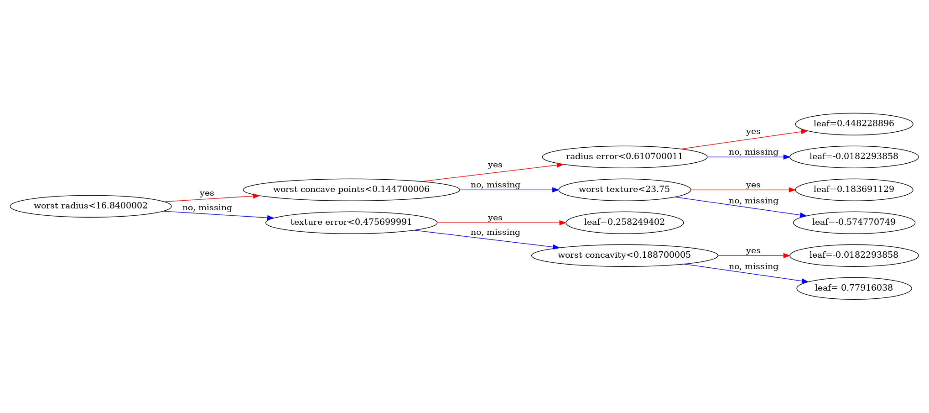
Figure 5: First booster tree (num_trees=0) of an xgb.XGBClassifier trained with binary:logistic, max_depth=3, and tree_method="hist" on the Wisconsin breast-cancer dataset, rendered via xgb.plot_tree / xgb.to_graphviz. Each internal node shows a feature, a numerical threshold (e.g. worst perimeter < 105.95), and a missing-value direction (yes or no/missing); each leaf shows its margin contribution leaf=....

How to read the tree in Figure 5:

• Internal nodes show <feature> < <threshold> plus a yes or no/missing = <node_id> line. The missing direction is the one XGBoost picks for rows where that feature is NaN — the sparsity-aware split selection from the original Chen & Guestrin paper.

• Leaves show leaf=<value>. That value is exactly \(w_j^* = -G_j / (H_j + \lambda)\) scaled by learning_rate. Sum the leaves you land in across all trees in the ensemble, add the base score, then apply sigmoid for binary:logistic (or softmax for multi:softprob) to get a probability.

• Following one row through the tree mirrors what PredictKernel does on the GPU: one thread per row walks the structure (broadcast through shared memory), accumulating leaf values. For an ensemble it does this K times in parallel and sums.

If you want to inspect the structure programmatically rather than visually, clf.get_booster().get_dump(dump_format="json") returns the same information as a list of JSON strings (one per tree), which the JSON model serializer writes to disk and every binding round-trips through.

Summary

This deep dive connected the math of XGBoost to the code that runs it. Part 1 derived gradient boosting from first principles: each tree fits the negative gradient of the loss, second-order Newton boosting falls out of a Taylor expansion, the regularized objective yields the closed-form leaf weight \(w_j^* = -G_j/(H_j+\lambda)\) and the Gain formula, and swapping only (g_i, h_i) turns the same algorithm into a regressor, a classifier, a ranker, or a survival model. Part 2 walked the library that implements it: the layered architecture from language bindings down to the tree engine, the C++ anchors for training and prediction, the five tree updaters and how tree_method and device select between them, the GPU kernels and data layouts (DMatrix, QuantileDMatrix, EllpackPage) behind tree_method="hist" on AMD Instinct GPUs, and a worked example that trained a real model and rendered its first booster tree.

Use this knowledge to move faster on your own workloads. When you tune gamma, reg_lambda, min_child_weight, or max_bin, you now know the exact term each one touches in the Gain formula, so you can reason about a change instead of running a blind sweep. When a run is slower or hungrier for memory than you expect, you can profile it with rocprof, recognize StHistKernel as the expected hot spot, and trace the cost back to bin count, tree depth, or a DMatrix choice that forces host round-trips. When you hit a wall that no parameter fixes, you can register a custom objective or metric through the plugin hooks and leave the boosting loop untouched. And when you read a stack trace, you can follow it from Learner::UpdateOneIter down to a kernel dispatch and explain what every layer is doing which is the skill that separates guessing from debugging.

Disclaimers

The information presented in this document is for informational purposes only and may contain technical inaccuracies, omissions, and typographical errors. The information contained herein is subject to change and may be rendered inaccurate for many reasons, including but not limited to product and roadmap changes, component and motherboard version changes, new model and/or product releases, product differences between differing manufacturers, software changes, BIOS flashes, firmware upgrades, or the like. Any computer system has risks of security vulnerabilities that cannot be completely prevented or mitigated. AMD assumes no obligation to update or otherwise correct or revise this information. However, AMD reserves the right to revise this information and to make changes from time to time to the content hereof without obligation of AMD to notify any person of such revisions or changes. THIS INFORMATION IS PROVIDED ‘AS IS.” AMD MAKES NO REPRESENTATIONS OR WARRANTIES WITH RESPECT TO THE CONTENTS HEREOF AND ASSUMES NO RESPONSIBILITY FOR ANY INACCURACIES, ERRORS, OR OMISSIONS THAT MAY APPEAR IN THIS INFORMATION. AMD SPECIFICALLY DISCLAIMS ANY IMPLIED WARRANTIES OF NON-INFRINGEMENT, MERCHANTABILITY, OR FITNESS FOR ANY PARTICULAR PURPOSE. IN NO EVENT WILL AMD BE LIABLE TO ANY PERSON FOR ANY RELIANCE, DIRECT, INDIRECT, SPECIAL, OR OTHER CONSEQUENTIAL DAMAGES ARISING FROM THE USE OF ANY INFORMATION CONTAINED HEREIN, EVEN IF AMD IS EXPRESSLY ADVISED OF THE POSSIBILITY OF SUCH DAMAGES.

Third-party content is licensed to you directly by the third party that owns the content and is not licensed to you by AMD. ALL LINKED THIRD-PARTY CONTENT IS PROVIDED “AS IS” WITHOUT A WARRANTY OF ANY KIND. USE OF SUCH THIRD-PARTY CONTENT IS DONE AT YOUR SOLE DISCRETION AND UNDER NO CIRCUMSTANCES WILL AMD BE LIABLE TO YOU FOR ANY THIRD-PARTY CONTENT. YOU ASSUME ALL RISK AND ARE SOLELY RESPONSIBLE FOR ANY DAMAGES THAT MAY ARISE FROM YOUR USE OF THIRD-PARTY CONTENT.

AMD, the AMD Arrow logo, AMD Instinct, ROCm, and combinations thereof are trademarks of Advanced Micro Devices, Inc. Other product names used in this publication are for identification purposes only and may be trademarks of their respective companies. © 2026 Advanced Micro Devices, Inc. All rights reserved