Diffusion-based Atmospheric Downscaling on AMD Instinct GPUs#

In addition to forecasting, reconstruction is also a commonplace procedure in atmospheric and climate sciences. Reconstruction in this context generally means estimating and infilling missing data, most often due to lack of sensor coverage. The data could be missing spatially or temporally, that is from some regions or at certain times respectively. The data could also be present at some scales and missing at some other scales – for example satellite ice coverage data would have larger scales present but be missing smaller scales due to resolution limitations. Reconstructing these missing smaller scales is called downscaling in climate sciences.
The idea of downscaling is to combine the existing large-scale information with constraints from physics and observations to estimate what the data at smaller scales might plausibly be. The classical approaches to this problem are typically grouped under the terms dynamical and empirical or statistical downscaling. These methods are based on either numerical physical modelling or statistical correlations with observations, respectively. However, with the advent of high-performance GPUs and new models, machine-learning-based methods now comprise a third, rapidly developing approach to the downscaling problem. This is especially true for deep learning and diffusion based machine learning models, which have demonstrated cutting edge performance.
In this blog post, we will describe the downscaling problem and briefly discuss the classical approaches used to tackle it. Next we will outline the new, machine learning based approach, and how it relates to the classical methods. We will also describe a specific diffusion-based downscaling model, CorrDiff, developed by NVIDIA.
Lastly, we will demonstrate how to run CorrDiff inference on AMD Instinct GPUs. We will provide step-by-step instructions so you can try it out yourself, and also visualize your results using our simple Python programs.
Atmospheric Downscaling#
Atmospheric downscaling is an umbrella term for methods that use observed or calculated values of atmospheric quantities available on a coarse resolution scale to estimate the values on a finer resolution scale. Or in other words, downscaling estimates missing high-resolution features based on low-resolution features. This might sound like an impossible or at least a very difficult proposition, since if the data at fine scales is missing completely, could it not be nearly anything? In this case, the answer turns out to be “no”. There are fundamental restrictions to what high-resolution features can correspond to any low-resolution observation of the real atmosphere.
Firstly, the coarser low-resolution data limits what the missing high-resolution features can be, as when suitably averaged, the result must still agree with the existing low-resolution data. In this sense, the low-resolution data serves as boundary conditions. Secondly, all features in the high-resolution data must have come about by physical processes, which are not arbitrary, and for which we can use the low-resolution data as both initial values and boundary values as well. This creates a further strict restriction for the high-resolution features. As such, for a given set of low-resolution data, only some high-resolution counterparts are compatible, and of these, some are more likely than others. This is the informal basis for why downscaling methods work.
The classical downscaling methods that are based on these observations can be divided into two categories: dynamical and statistical. The dynamical methods emphasize the underlying physics for estimating the high-resolution features. On the other hand, statistical methods are based on regressing observed (or simulated) correlations between high-resolution and low-resolution features.
The newer machine learning based methods could also in principle be grouped with classical statistical methods since they formally work on the same principle. However, it is convenient to have them as a separate category, which is a typical approach in literature, and which we will also follow here. For a review on classical downscaling and machine learning based downscaling methods, see [2] and [3], respectively, and the references therein.
Dynamical downscaling#
The idea behind dynamical downscaling is to use low-resolution data from observations or simulations as the boundary and initial conditions for a high-resolution physical simulation. Typically this high-resolution simulation will only be run for a relatively short time, and is restricted to some local area of interest. Hence it will typically not incorporate interactions that are only relevant at large scales or longer times, such as a full ocean-atmosphere coupling.
The local simulation may start with initial conditions that are smooth, as determined by interpolating the low-resolution data. However, the increased resolution will allow modeling unresolved smaller scale effects like turbulence, convection, and the effects of orography. These will quickly cause the simulation to develop the initially missing high-resolution features.
There are some inherent drawbacks to dynamical downscaling. An obvious problem is the fact that running a very high-resolution physical simulation requires significant computational resources. This can place limits on the size of the region being downscaled, or generally on the number of downscaled datasets that can be computed in a given time.
On the other hand, the dynamical downscaling process is not fully physically consistent, as the full couplings to the large-scale environment are missing. For example, the local high-resolution simulation typically does not affect the sea surface temperatures, which are only used as inputs. In general, the information typically flows only from the low-resolution data to the high-resolution simulation, but not the other way around. This prevents larger scale features from being seeded by the smaller scale features in the high-resolution simulation, although this otherwise can happen in the chaotic climate system.
Statistical downscaling#
Statistical downscaling, sometimes also called empirical downscaling, is based on trying to statistically estimate the missing high-resolution small scale features using the low-resolution large scale features as predictors. This can be achieved through numerous methods that differ in detail, and which can be further categorized into families. Here we will only briefly mention some typical approaches.
For example, the change factor method mentioned above is perhaps the simplest method of this kind. In this method, the time evolution of a large scale simulation is directly used to scale existing observational high-resolution data to produce the downscaled results. The drawbacks are obvious, as all the model dynamics come from the low-resolution simulation, and thus no local systematic changes can be modelled.
A more advanced approach is to use some multivariate regression technique to estimate local smaller scale features from the local and surrounding larger scale features. There is an abundance of methods to choose from, such as simple multiple regression, principal component analysis, correlation analysis or even neural networks. The last option in particular will be discussed in detail below.
While statistical downscaling methods are in general much less computationally demanding than dynamical downscaling methods, they also do come with drawbacks. The key problem is that there is no guarantee that any estimated correlation or regression relation between large and small scale features survives the inevitable shifts of both local and global climate. Given how the methods are typically constructed, inter-variable dependencies and extremal values may also not come out faithfully represented.
ML-based downscaling#
Downscaling based on machine learning could be called empirical or statistical as well, but the methods are sufficiently different to warrant a separate category. Deep learning methods and generative methods in particular have made it possible to reach high output accuracy coupled with estimation of output uncertainty, while still maintaining reasonable computational complexity.
The deep learning advances such as convolutional neural networks (CNNs) and the various transformer architectures make it feasible to learn highly non-linear end-to-end maps between low-resolution inputs and high-resolution outputs. These models can also process two-dimensional and three-dimensional data in a natural way that respects the underlying geometric structure of the data.
On the other hand, new generative methods such as diffusion models can be used to obtain estimates of the output uncertainty without the computational burden of doing a full Bayesian end-to-end computation. The generative methods can also naturally provide ensembles of possible output realizations. These can retain high-frequency, low-probability features that would otherwise get smoothed out by the averaging in any purely mean-based prediction.
For a comprehensive review on recent machine learning based advances in downscaling see for example [3] and the references therein. Similarly, see [4] for a general overview of machine learning based advances in weather modeling.
CorrDiff#
CorrDiff (short for Correction Diffusion) is a convolutional, diffusion-based downscaling method developed by the NVIDIA Corporation. The full technical details are presented in the publication [1], and the model itself can be obtained for example as a part of the Earth2Studio framework, released under Apache License 2.0.
The model consists of two stages. The first stage is a deterministic, convolutional U-Net-based predictor, which produces high-resolution mean estimates from lower resolution ERA5 reanalysis data. The second stage is a diffusion model based corrector, which samples from a distribution of residuals between the predicted mean state and the unobserved ‘true’ output.
This model structure is quite similar to the one used in StormCast, NVIDIA’s high-resolution weather prediction model. We have discussed StormCast and its similar two-step structure in more detail previously in two separate blog posts: High-Resolution Weather Forecasting with StormCast on AMD Instinct GPU Accelerators and Ensemble High-Resolution Weather Forecasting on AMD Instinct GPU Accelerators. The main difference between the two models is that StormCast infers a sequence of future high-resolution weather states autoregressively, whereas CorrDiff is focused on inferring high-resolution detail from low-resolution input. Overall, this two-stage structure is not limited to CorrDiff and StormCast. For example, GeoArches is based on a similar approach, and you can read more about it in another previous blog post: Training AI Weather Forecasting Models on AMD Instinct.
The model as published was designed and trained to work in a compact region surrounding Taiwan. The input format is a \(32\times 32\) grid of 12 ERA5 reanalysis quantities consisting of wind, geopotential, temperature and water vapor both on the surface and vertically. The output is a \(448\times 448\) super-resolution grid of surface quantities, namely east and north wind components, temperature and maximum radar reflectivity (a proxy for precipitation).
The publication [1] shows that the complete, trained CorrDiff model exhibits superior performance compared to a set of baseline models, namely interpolation of low-resolution ERA5 data, a Random Forest model and the bare deterministic, regression part of CorrDiff itself. This was found to be the case with respect to a typical indicator of predictive skill, namely Continuous Ranked Probability Score (CRPS), which reduces to Mean Absolute Error (MAE) for the deterministic baseline methods. The superior performance of CorrDiff was also demonstrated with respect to the power spectra and probability distributions of the outputs.
The deterministic part#
The deterministic part of CorrDiff is a U-Net model. This is a convolution network that first contracts the input from image space to feature space, and then expands from the feature space back to the desired resolution. The essential innovation is the use of long-range skip connections, which connect the convolutional layers of similar resolution. This part of the CorrDiff model contains approximately \(79.7\) million parameters.
The deterministic part is trained to predict a mean high-resolution output \(\mu\), where we should understand this to be the mean with respect to the uncertainty of the output. For the published model, the training itself was done using the high-resolution data from the Central Weather Administration (CWA) of Taiwan. The data was produced using a dynamical downscaling approach combined with radar observations.
The diffusion model#
The key innovation in CorrDiff is the use of a diffusion model to ‘correct’ the mean prediction obtained from the deterministic U-Net stage. For a condensed explanation on how diffusion models work, please see our previous blog post. The diffusion model used in CorrDiff contains approximately \(80.0\) million parameters.
Essentially, the diffusion model is trained to predict the uncertainty around the output mean in a distributional sense, conditioned on the low-resolution input. The model can then sample corrections \(r\) from this distribution, which by construction should be very close to zero-mean. The sampled combinations \(\mu + r\) then form an ensemble of possible outputs, and the ensemble should closely model the distribution of plausible high-resolution outputs given the low-resolution input.
Installation#
For following the instructions below, you will need the following at a minimum:
A computer with an AMD Instinct GPU. The examples in this blog post were run on an MI300X.
A GNU/Linux operating system with Docker® installed.
ROCm kernel driver installed. See the instructions for running ROCm Docker containers.
Note
As with our previous blog posts, we have provided two Python programs to simplify the use of CorrDiff. You should download run-corrdiff.py and plot-corrdiff.py and place them in your working directory. These files contain all of the code examples from below and more, so you may wish to use their contents to further help you understand the material to follow.
The easiest way to get CorrDiff running on AMD Instinct hardware is to use a ROCm Docker image.
For the examples in this blog post we have used the image
rocm/pytorch:rocm7.0.2_ubuntu24.04_py3.12_pytorch_release_2.8.0. If you have
Docker installed on your system, you can download this image simply by invoking the following:
docker pull rocm/pytorch:rocm7.0.2_ubuntu24.04_py3.12_pytorch_release_2.8.0
The recommended way to spin up the image in a container is to use the AMD Container Toolkit. If you have it installed, you can spin up a container with the following command:
docker run -d \
    --runtime=amd \
    -e AMD_VISIBLE_DEVICES=all \
    --name corrdiff \
    -v $(pwd):/workspace/ \
    rocm/pytorch:rocm7.0.2_ubuntu24.04_py3.12_pytorch_release_2.8.0 \
    tail -f /dev/null
If you do not have the AMD Container Toolkit installed, you can run the following command instead:
docker run -d \
    --device=/dev/kfd \
    --device=/dev/dri \
    --group-add video \
    --name corrdiff \
    -v $(pwd):/workspace/ \
    rocm/pytorch:rocm7.0.2_ubuntu24.04_py3.12_pytorch_release_2.8.0 \
    tail -f /dev/null
Note
In the above, we’ve assumed that you’ve downloaded the helper programs and
anything else you wish to have available in the container to your current
working directory. Both Docker commands above will map your working directory
into the directory /workspace inside the container.
When the container is running, you can now open a new interactive shell in the container by running the following:
docker exec -it corrdiff /bin/bash
In the new session, move to the workspace directory and install the required Python dependencies by running the following:
cd /workspace
pip install earth2studio[corrdiff] cartopy
You now have a running container with a fresh CorrDiff installation!
Running CorrDiff#
Running CorrDiff inference from Python is slightly more involved than the code examples in our previous StormCast blog posts. There is no reason to worry however, as we will introduce everything in easily understandable pieces below.
Note
Depending on your specific setup, you may encounter warnings like
DeprecationWarning: The symbol warp.context.Device will soon be removed from the public API. Use warp.Device instead. while running some parts of the code
below. These are internal to libraries used by Earth2Studio, and in our
experience you should be able to safely ignore these. The code should still run
on your GPU (or CPU) without problems.
To begin, you will need the following imports.
import os
import shutil
from collections import OrderedDict

import numpy as np
import pandas as pd
import torch
from earth2studio.data import GFS, prep_data_array
from earth2studio.io import ZarrBackend
from earth2studio.models.dx import CorrDiffTaiwan
from earth2studio.utils.coords import map_coords, split_coords
You will also need a number of helper functions for managing the input and output data. We define these next. Note that these same definitions can be found in the program run-corrdiff.py, but with type information and comments added to help you understand what the functions do.
def create_output_file(template):
    os.makedirs('outputs', exist_ok=True)
    outf = os.path.join('outputs', template)
    if os.path.exists(outf):
        print(f'Removing existing output {outf}')
        try:
            shutil.rmtree(outf)
        except Exception as e:
            print(f'Error removing directory {outf}: {e}')

    return ZarrBackend(outf), outf


def fetch_input_data(device, data_source, model, starting_datetime):
    input_data = data_source([starting_datetime], model.input_coords()['variable'])
    x, coords = prep_data_array(input_data, device=device)
    x, coords = map_coords(x, coords, model.input_coords())

    return x, coords


def setup_output(io, data_input_coords, model):
    output_coords = model.output_coords(model.input_coords())
    total_coords = OrderedDict(
        {
            'time': data_input_coords['time'],
            'sample': output_coords['sample'],
            'lat': output_coords['lat'],
            'lon': output_coords['lon'],
        }
    )
    io.add_array(total_coords, output_coords['variable'])

    return io
With these definitions, we can run CorrDiff for a given datetime by doing the following. First, we set up the target date and time.
npdatetime = np.datetime64('2024-07-24T12:00')
starting_datetime = pd.to_datetime(npdatetime).to_pydatetime()
date = npdatetime.astype('datetime64[D]')
This slightly convoluted call lets us use a string input to set
the variable starting_datetime to 24th of July 2024, 12:00 UTC, and the
variable date to just the corresponding date without the time. This happens to
be the date and time during which the
Typhoon Gaemi
was over the island of Taiwan.
Next we need to set up the output file. The output will be stored as a Zarr
container in the directory outputs/ under the working directory. This Zarr
container is not a single file, but instead it consists of an entire directory
structure, which defines the contents of the container.
See the Zarr documentation for further details.
Our particular example will be stored in outputs/corrdiff-2024-07-24.zarr/.
output_template = f'corrdiff-{date}.zarr'
io, output_fname = create_output_file(output_template)
Then we need to set up the CorrDiff model itself and define a data source. The model weights can be directly obtained using the Earth2Studio functionality. Note that while the model was trained using ERA5 data, with Earth2Studio we can use other global low-resolution models as input as well. Here we use the GFS (Global Forecast System) synoptic scale reanalysis data by the National Oceanic and Atmospheric Administration (NOAA) as the data source. The main reason is that the GFS data in Earth2Studio extends to the present date, but the Earth2Studio ERA5 support does not.
Note
Running the following will download data (the model weights) from the Internet to the machine where you are running the command.
data_source = GFS()

package = CorrDiffTaiwan.load_default_package()
model = CorrDiffTaiwan.load_model(package)
Next we finalize setting up the model by moving it to the Torch device and
setting the number of samples in our ensemble we will generate. Note that
increasing the samples will increase the fidelity with which the generated
ensemble will capture the predicted uncertainty, but it will also linearly
increase the inference time.
If everything has gone right, running the code below should print cuda.
device = torch.device('cuda' if torch.cuda.is_available() else 'cpu')
model.to(device)
print(f'Running CorrDiff on device: {device}')

# Decrease this if the inference time is too large, or increase this to increase fidelity.
model.number_of_samples = 4
As the last thing before running the model we need to download the input data and setup the output.
Note
Running the command below will also download data (the input weather data) from the Internet to the machine where you are running the command.
x, coords = fetch_input_data(device, data_source, model, starting_datetime)

io = setup_output(io, coords, model)
Now we can run the model and save the output. Note that since CorrDiff is what
is called a diagnostic model in the Earth2Studio nomenclature, we run it simply
by invoking the model object’s __call__() function.
x, coords = model(x, coords)

io.write(*split_coords(x, coords))
This will compute a downscaled version of the GFS data for the given date and store the result into the Zarr storage we set up above. The output will contain eastward and northward wind components at the height of 10 meters, temperature at 2 meters and the maximum radar reflectivity.
Running this example with four ensemble members on an MI300X GPU was observed to use around 4% of VRAM at the peak, or 7.5 GB. Wallclock time taken to run the inference after the model weights have been downloaded was roughly 30 seconds. The memory usage and elapsed inference time scale approximately linearly with the number of ensemble samples chosen, for a smallish amount of samples from 1 to 16.
Instead of writing all of the above, you can just use the run-corrdiff.py program we have provided. Using this program, you can achieve the same result by invoking it with the following.
python run-corrdiff.py 2024-07-24T12:00 --samples 4
Try also using the --help command line option to get more information on how
to use the program.
Next, let’s see what we can do about plotting the results we have obtained.
Plotting the results#
For plotting the downscaled result, we will need some further imports. As is
typical, we will use matplotlib as the plotting backend with cartopy for the
cartographic projections.
import cartopy.crs as ccrs
import matplotlib.pyplot as plt
import xarray as xr
First we need to open the saved zarr output and extract the number of samples and the date.
fname = 'outputs/corrdiff-2024-07-24.zarr'
ds = xr.open_zarr(fname, consolidated=False)
sample_indexes = np.arange(len(ds['sample'].to_numpy()))
datetime = ds['time'].to_numpy()[0]
date = datetime.astype('datetime64[D]')
Next we need to set up the projection and transform to match the original CorrDiff publication. The publication indicates that the data is plotted using the Lambert Conformal Conical projection centered on the island of Taiwan. Here we will use the center point of the latitude and longitude ranges as given in the publication.
In addition we need to define a projection, which matplotlib will use to
transform the input coordinates to the output projection. The stored CorrDiff
output is in latitude-longitude pairs, so the correct projection is the
PlateCarree projection, which matches this coordinate definition.
For more information,
see this explanation
at the yt project.
lat_mid = 0.5 * (19.5483 + 27.8446)
lon_mid = 0.5 * (116.371 + 125.568)
projection = ccrs.LambertConformal(central_longitude=lon_mid, central_latitude=lat_mid)
map_transform = ccrs.PlateCarree()
With these preliminaries out of the way, we can now create and save a figure for each sample contained in the ensemble by looping over the samples. Each figure will have a horizontal row of three panels containing heatmaps of the radar reflectivity, temperature and wind speed, respectively. In addition, the last panel will have wind direction and speed superimposed as arrows of varying length and direction. All this can be achieved with the following lengthy snippet.
colormap = 'magma'
for sample_ix in sample_indexes:
    figsize = (15, 6)
    fig, _ad = plt.subplot_mosaic(
        'abc',
        per_subplot_kw={
            'a': dict(projection=projection),
            'b': dict(projection=projection),
            'c': dict(projection=projection),
        },
        figsize=figsize,
        layout='compressed',
    )
    axes = np.array([_ad['a'], _ad['b'], _ad['c']])

    # There are only four quantities predicted by CorrDiff.
    # The quantities are indexed in the output by the following strings,
    # which we use in the following:
    # - mrr: Maximum radar reflectivity [dBz]
    # - t2m: Temperature at 2m height [C].
    # - u10m: Wind U component at 10m height [m/s].
    # - v10m: Wind V component at 10m height [m/s].

    # Plot maximum radar reflectivity.
    pmesh = axes[0].pcolormesh(ds['lon'], ds['lat'], ds['mrr'][0, sample_ix], transform=map_transform, cmap=colormap)
    plt.colorbar(pmesh, ax=axes[0], label='Radar reflectivity [dBz]')

    # Plot temperature.
    pmesh = axes[1].pcolormesh(
        ds['lon'], ds['lat'], ds['t2m'][0, sample_ix] - 273.15, transform=map_transform, cmap=colormap
    )
    plt.colorbar(pmesh, ax=axes[1], label='Temperature at 2m [deg C]')

    # For the wind vectors, we need decimated data.
    lons = ds['lon'].to_numpy()
    lats = ds['lat'].to_numpy()
    wind_u = ds['u10m'][0, sample_ix].to_numpy()
    wind_v = ds['v10m'][0, sample_ix].to_numpy()
    wind_speed = np.sqrt(wind_u**2 + wind_v**2)

    # Decimate by a factor of df.
    df = 6
    dec_lons = lons[::df, ::df]
    dec_lats = lats[::df, ::df]
    dec_u = wind_u[::df, ::df]
    dec_v = wind_v[::df, ::df]

    # Plot wind speed and velocity vectors.
    pmesh = axes[2].pcolormesh(ds['lon'], ds['lat'], wind_speed, transform=map_transform, cmap=colormap)
    plt.colorbar(pmesh, ax=axes[2], label='Wind speed [m/s]')
    axes[2].quiver(dec_lons, dec_lats, dec_u, dec_v, transform=map_transform, width=5e-4)

    # Add coastlines and grid lines to each panel.
    for ax in axes:
        ax.gridlines(draw_labels=True, dms=True, x_inline=False, y_inline=True, alpha=0.5)
        ax.coastlines()

    # Add a title with the date. Use pandas Timestamp for more readable string representation.
    fig.suptitle(f'CorrDiff sample {sample_ix} for t={pd.to_datetime(datetime)}')

    # Save the plot.
    output_fname = f'corrdiff-{date}-sample-{sample_ix}.jpg'
    print(f'Saving plot to {output_fname}')
    plt.savefig(output_fname)
Running this snippet will create one figure for each sample, and store them in
the working directory under the names corrdiff-[date]-sample-[sample index].jpg.
For our particular example, the stored files will be from
corrdiff-2024-07-24-sample-0.jpg to corrdiff-2024-07-24-sample-3.jpg.
The figures will contain all the outputs produced by CorrDiff, namely maximum radar reflectivity, temperature at the height of two meters, and the East and North components of the wind velocity at the height of 10 meters. The radar reflectivity and the temperature are depicted as heatmaps in the left and center panels, respectively. The rightmost panel depicts the wind velocity components as small arrows indicating the wind direction and magnitude or speed. The wind speed is also depicted as a heatmap in the rightmost panel.
An example is shown below in Figure 1. In the figure, the structure of the Typhoon Gaemi is clearly visible both in the leftmost panel (max. radar reflectivity) and the rightmost panel (wind speed). The typhoon can be seen to cover the entire island of Taiwan with the eye of the typhoon being roughly situated on the eastern coast of Taiwan.
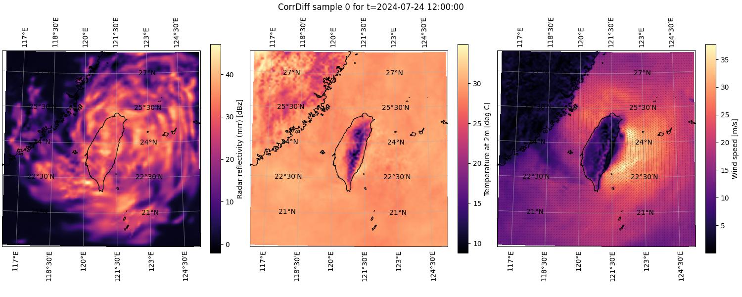
Figure 1. The first sample in an ensemble of CorrDiff results computed for 2024-07-24 at 12:00 UTC. The left and center panels depict heatmaps of the scalar quantities maximum radar reflectivity and temperature at a height of 2 meters, respectively. The right panel depicts wind speed at 10 meters as a heatmap and the corresponding wind direction as small arrows.#
Perhaps the easiest way to visualize the uncertainty in the ensemble of results is by combining the outputs into an animation. If you have the common ImageMagick® software package installed, you can create an animation of the plotted outputs by simply running the following command.
convert -loop 0 -delay 100 corrdiff-2024-07-24-sample-*.jpg corrdiff-animation.gif
This command will create the file corrdiff-animation.gif, which contains an
animation that will continuously loop through the plots of all the samples in
the ensemble. You can see this animation below in Figure 2.

Figure 2. Animation cycling through all of the CorrDiff results computed and plotted for 2024-07-24 at 12:00 UTC. See the caption of Figure 1 for details on the component plots.#
We can further compare the CorrDiff outputs to the corresponding quantities from
the GFS low-resolution data that is being used as the CorrDiff input. In Figure 3 below
we’ve plotted the same quantities as in Figures 1 and 2 with the exception of
having replaced maximum radar reflectivity (mrr) with the composite radar
reflectivity (refc), as the former is not available in GFS.
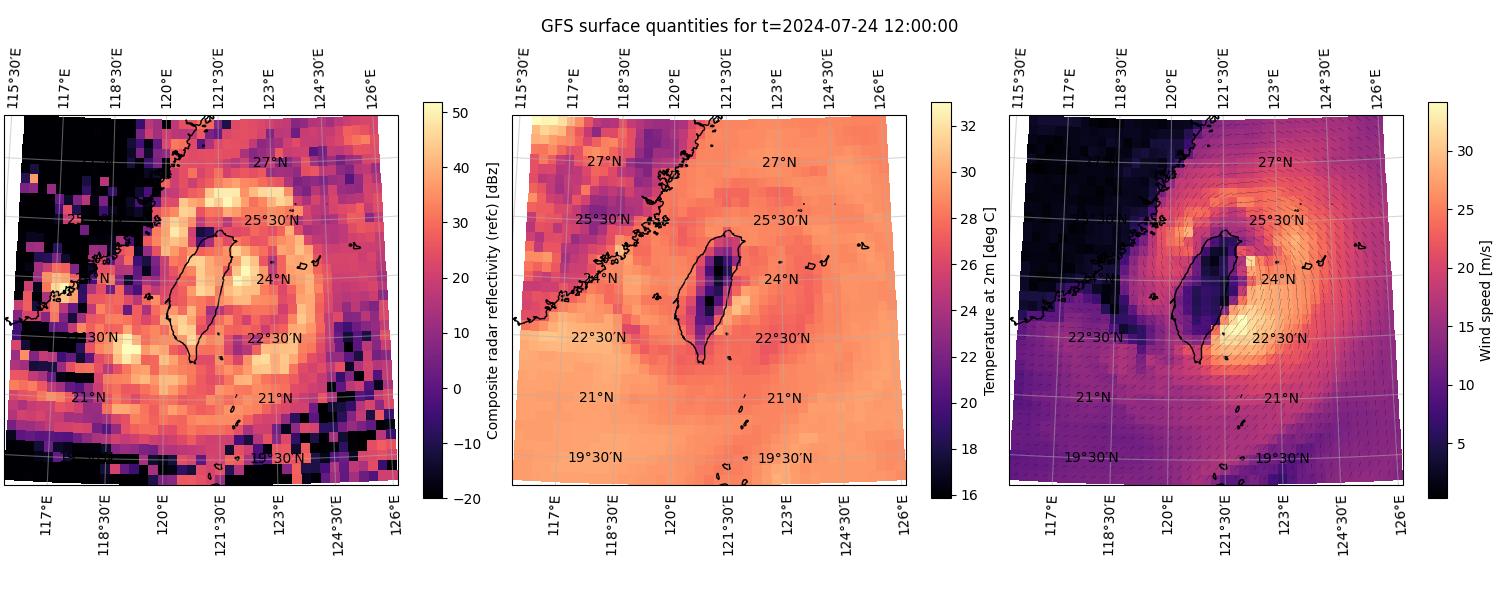
Figure 3. Selected GFS variables retrieved for 2024-07-24 at 12:00 UTC. The left and center panels depict heatmaps of the scalar quantities composite radar reflectivity and temperature at a height of 2 meters, respectively. The right panel depicts wind speed at 10 meters as a heatmap and the corresponding wind direction as small arrows.#
Again, note that you can also achieve the same plots by just using the plotting program plot-corrdiff.py, which accompanies this blog post. Using this program, you can create the same plots as with the code above just by running it as follows.
python plot-corrdiff.py outputs/corrdiff-2024-07-24.zarr --plot-lowres
This invocation will plot both all the CorrDiff samples in the output ensemble
as well as the corresponding low-resolution GFS data. Again, try using the
--help command line option to see more documentation and ways to use the
program.
Summary#
Measurements, simulations and machine learning based inference of weather are naturally limited in resolution by either sensor coverage or computational resources, respectively. One way around this limitation is to use atmospheric downscaling, in which we locally infer the most likely high-resolution state that corresponds to the lower resolution data we do have. In a more formal sense this means inferring missing high frequency scales from available low frequency data.
In this blog post we have described the downscaling problem and discussed some common approaches to solving it. In particular, we have presented CorrDiff, a machine learning based downscaling method that directly transforms low-resolution meteorological reanalysis data to high-resolution surface quantities. The model is also capable of estimating the uncertainty of the predictions via ensembles obtained through a diffusion process.
We demonstrated how to set up and run the CorrDiff model on AMD Instinct GPUs using simple, straightforward code snippets. Similarly, we demonstrated how the outputs can be plotted with a few lines of Python code. We also provided two Python programs that can be used to run the model and plot the results without the need for any coding on the reader’s part.
We hope you have found the discussion and the tips interesting, and urge you to check out our previous blog posts discussing diffusion based weather models. Currently this series consists of the following: High-Resolution Weather Forecasting with StormCast on AMD Instinct GPU Accelerators and Ensemble High-Resolution Weather Forecasting on AMD Instinct GPU Accelerators.
Additional Resources#
The CorrDiff runner program: run-corrdiff.py
The CorrDiff plotter program: plot-corrdiff.py
The thumbnail image is from AMD stock imagery collection.
License#
CorrDiff is released bundled with Earth2Studio, under the Apache License 2.0. Please see the full text of the license.
Docker and the Docker logo are trademarks or registered trademarks of Docker, Inc.
ImageMagick is a trademark of ImageMagick Studio LLC.
References#
[1] Mardani, M., Brenowitz, N., Cohen, Y. et al. (2024). Residual Corrective Diffusion Modeling for Km-scale Atmospheric Downscaling. arXiv:2309.15214
[2] Ekström, M., Grose, M. R., & Whetton, P. H. (2015). An appraisal of downscaling methods used in climate change research. Wiley Interdisciplinary Reviews: Climate Change, 6(3), 301-319. https://doi.org/10.1002/wcc.339
[3] Rampal, N., Hobeichi, S., Gibson, P. B., et al. (2024). Enhancing regional climate downscaling through advances in machine learning. Artificial Intelligence for the Earth Systems, 3(2), 230066. https://doi.org/10.1175/AIES-D-23-0066.1
[4] Bracco, A., Brajard, J., Dijkstra, H. A., et al. (2025). Machine learning for the physics of climate. Nature Reviews Physics, 7(1), 6-20. https://doi.org/10.1038/s42254-024-00776-3
Disclaimers#
Third-party content is licensed to you directly by the third party that owns the content and is not licensed to you by AMD. ALL LINKED THIRD-PARTY CONTENT IS PROVIDED “AS IS” WITHOUT A WARRANTY OF ANY KIND. USE OF SUCH THIRD-PARTY CONTENT IS DONE AT YOUR SOLE DISCRETION AND UNDER NO CIRCUMSTANCES WILL AMD BE LIABLE TO YOU FOR ANY THIRD-PARTY CONTENT. YOU ASSUME ALL RISK AND ARE SOLELY RESPONSIBLE FOR ANY DAMAGES THAT MAY ARISE FROM YOUR USE OF THIRD-PARTY CONTENT.