DI Series: Serving Kimi-K3 MXFP4 Wide-EP Disaggregated on AMD Instinct MI300X and MI325X

DI Series: Serving Kimi-K3 MXFP4 Wide-EP Disaggregated on AMD Instinct MI300X and MI325X#

October 08, 2026 by Ravi Gupta, Mir Ali, Doug Lehr, Basem Barakat, Markus Hartikainen, Nico Holmberg, Vikram Appia, Anuj Mittal, Onil Gunawardana, Aswin Mathews, Peng Sun, Emad Barsoum.

44 min read. | 10815 total words.

Software tools & optimizations

AI/ML, LLM, Performance, Serving, Optimization, Memory

AI, Systems

This post is part of the AMD Disaggregated Inference (DI) Blogs Series, which takes frontier open models from a single-node demo to production, multi-node serving on AMD Instinct™ GPUs

Kimi-K3 in MXFP4 (Microscaling FP4) occupies 1453.7 GiB of weights, while an eight-GPU AMD Instinct™ MI300X node provides approximately 1504 GiB of usable high-bandwidth memory. A single resident weight replica therefore leaves roughly 50 GiB across the entire node (for the key-value (KV) cache, the activations, and the communication heap combined). That margin is insufficient in practice: a conventional single-node deployment cannot allocate a KV pool large enough to generate tokens at useful sequence lengths.

This is the first of three constraints. MXFP4, the quantization format that makes a 2.8-trillion-parameter Mixture-of-Experts (MoE) model tractable, has no native matrix-multiply instruction on the CDNA 3 (gfx942) architecture common to MI300X and MI325X. A serving stack pointed at the checkpoint does not fail, but it cannot use the format directly either, so the experts have to be requantized into a format the matrix engine accelerates, and that choice decides whether the memory saving survives. The third constraint is architectural: Kimi-K3 is a hybrid in which only 24 of its 93 layers use Multi-head Latent Attention (MLA), and the remaining 69 use gated-delta recurrent Kimi Delta Attention (KDA). The prefill-to-decode handoff must therefore transport a recurrent state alongside the KV cache, over a path that a pure-attention model never exercises, and that path was found to contain two correctness defects.

A single deployment shape resolves all three constraints. Prefill and decode execute on separate GPU pools, the 896 routed experts are sharded sixteen ways, the attention stack that cannot be expert-sharded is split two ways and replicated eight ways, and the AMD MoRI stack provides both the expert all-to-all and the remote direct memory access (RDMA) cache transfer within vLLM. This post establishes why that shape follows from the memory arithmetic and not from preference, identifies the kernel substitution that makes an MXFP4 checkpoint execute efficiently on gfx942, and documents how the two concurrency defects were diagnosed and corrected before any performance measurement was accepted. It then characterizes the deployment: recall accuracy at long context, a concurrency envelope on both platforms, replay of recorded agentic traces with AgentX, and a capacity model that converts a service-level agreement (SLA) into a node count, a context ceiling, and a concurrency limit before hardware commitment.

About this series. This post is the second in the AMD Disaggregated Inference (DI) Blog Series, which takes open frontier models from a single-node demo to multi-node serving on AMD Instinct™ GPUs. The first post, Scaling GLM-5.1-FP8 to 64 MI300X GPUs, covers the same disaggregated wide expert-parallel approach on a different model. Each post in the series follows one model from the memory arithmetic that decides its deployment shape through to measured serving behavior, and more are to follow.

In this post you will learn how to serve a 1.4 TiB MXFP4 mixture-of-experts checkpoint across two prefill and two decode nodes. Specifically, you will see:

Why the memory budget forces that deployment shape, rather than leaving it to preference.
Which kernel substitution makes MXFP4 run efficiently on an architecture with no native MXFP4 instruction.
How two concurrency-correctness defects were found and fixed before any performance number was accepted.
How to turn a service-level agreement into a node count, a context ceiling, and a concurrency limit, using a capacity model you can compute before committing hardware.

At a Glance#

The following points summarize the main results in this post:

Enabled: Kimi-K3 MXFP4 served as 2P2D disaggregated, wide expert-parallel (EP16) in vLLM on both MI300X (192 GB, ConnectX-7) and MI325X (256 GB, Broadcom Thor2 RoCE).
Two correctness defects found and fixed: a MoRIIO RDMA KV write-race and a KDA recurrent-state recycle bug. After both fixes, distinct-needle recall under concurrency is 57 of 57 on both platforms.
The MXFP4-on-gfx942 wall is solved via an int4-SiTU (SiTUv2 a8w4) MoE path, because the native MXFP4 kernel does not exist on this architecture.
A decode-side capacity model, validated: per-token decode speed is comparable across the two platforms, at 74 against 82 ms/token, so compute is not what separates them. Capacity is, and it is worth being precise about which capacity: MI325X rides the concurrency floor to concurrency 512 (1235 tokens/s) while MI300X plateaus at concurrency 64. That plateau is the in-flight sequence-slot count, MAX_NUM_SEQS times the eight data-parallel lanes, and a controlled run proves the mechanism: raising MAX_NUM_SEQS from 8 to 32 on the same MI300X pool moves the knee and lifts throughput at concurrency 128 by 28%, so it is a setting, not a hardware limit. The KV pool takes over as the binding constraint at long context, where it sets a 3.1x concurrency gap.
Context frontier: both platforms recall a needle at 900K tokens, and neither ceiling is set by KV capacity. Each stops at its configured max_model_len, 1,000,000 on MI325X and 900,000 on MI300X, with the MI300X decode pool holding more tokens than the limit it was given.
Validated on long-context agentic traffic, not only on synthetic shapes: multi-turn session traces replay to a 244K-token input p99 on both platforms and 414K on MI325X, with sessions running to 103 and 144 turns and prefix reuse near 90%, and every profile completing with no in-window wire errors. At concurrency 1 the same replay reproduces the per-token cost the capacity model predicts to within 3 to 5%, so the model holds under real traffic and not only under fixed request shapes.

A single request moves through the deployment in three acts, and Figure 1 below animates one.

Act 1, prefill. Eight concurrent requests each own one data-parallel lane, because a lane is an independent replica rather than a slice of one request. The 24 MLA and 69 KDA layers cannot be expert-sharded, so every prompt token is processed inside its own lane: the two GPUs of a lane split the work with tensor parallelism (TP2) and reduce across the pair, giving TP2 x DP8 = 16 attention ranks at 53.3 GiB per GPU. Attention writes the cache as it goes. The router then assigns each token the experts it needs, and the tokens queue at the boundary. The 896 routed experts are sharded 16 ways (EP16), 56 experts and 84.2 GiB per GPU, so a token must travel to whichever GPU owns its expert. That is the MoRI-EP all-to-all: dispatch to the owners, then combine the partial results back to the home lane. Three of every sixteen tokens find their expert inside their own lane and never leave it. All of this repeats for 93 layers.

Act 2, transfer. The finished cache, 13.8 MiB per request at an input length of 1024 tokens, crosses to the decode pool. MoRIIO performs a one-sided GPU-Direct RDMA write carrying both the MLA latent KV cache and the KDA recurrent state, at 14,098 bytes per token. That single hop is the disaggregation tax inside time to first token, and completing it frees the prefill GPUs for the next prompt.

Act 3, decode. The decode pool runs the same TP2 x DP8 attention and the same EP16 experts, but the rhythm inverts: one token per sequence per step, each new token appended to the cache and fed back as the next input, at roughly 74 ms per step on MI325X. Whatever high-bandwidth memory (HBM) is left after weights, heap, and graph capture becomes the KV pool, 40 GB on MI325X and 13 GB on MI300X. Much of this post is about what that number does and does not determine.

Figure 1. One request’s journey through the 2P2D deployment, animated in three acts: prefill, the cache transfer, and decode. The stage indicator at the top tracks which act is running, and the line along the bottom explains each step as it happens. The token routing shown is illustrative and not captured from a live trace.

Why Disaggregate, and Why Wide Expert Parallelism#

Large language model (LLM) inference has two phases with opposite personalities. Prefill ingests the prompt: it is compute-bound, processes all prompt tokens in parallel, and runs in bursts. Decode emits the answer one token at a time: it is latency-bound and memory-bandwidth-bound, and it runs as a long stream. Co-locating both on the same GPUs forces one set of kernels and one scheduling regime to serve two workloads with different bottlenecks, and the bursty prefill interferes with the steady decode stream.

Prefill-decode (PD) disaggregation (the “DI” in this series) puts prefill and decode on separate pools of GPUs and streams the KV cache between them. Each pool can then be tuned for its own phase: the prefill pool runs a high-throughput all-to-all and eager execution, while the decode pool runs a low-latency all-to-all and captures graphs.

Wide expert parallelism is the other half. Kimi-K3 routes each token to 16 of 896 experts, and there are two ways to place them. Tensor-parallel placement splits each expert general matrix multiply (GEMM) into N smaller fragments, which are memory-bound, and every layer pays an all-reduce that does not amortize with batch size. Expert-parallel placement gives each GPU a full-size subset of experts and routes tokens to wherever their experts live, so the GEMMs stay full-size and attention batches well. That’s why this recipe is wide-EP, with the experts EP16-sharded in every viable layout.

EP16 also fixes the shape of the deployment. Sixteen expert ranks across 8-GPU nodes means two nodes per pool, so 2P2D, two prefill nodes and two decode nodes, is the smallest disaggregated wide-EP configuration that can hold the model at all. It is a floor, not a tuned ratio, and one of the results below suggests the prefill half of it is the side under more pressure.

The all-to-all adds a fixed per-wave latency floor set by fabric bandwidth. Because that floor is fixed and not per-request, concurrency is close to free while requests keep fitting, which is the property the rest of this post tests. What stops them fitting is the more interesting question, and the answer is not the one the memory arithmetic suggests.

The Model: A KDA, MLA, and MoE Hybrid#

The following table lists the model properties that shape every decision in this post:

Property	Value
Total parameters	~2.8 T (896 routed experts, top-16 active, + 2 shared)
Weights on disk	1453.7 GiB (measured from the safetensors index)
Layers	93 total = 24 MLA (full attention) + 69 KDA (gated-delta recurrent)
MLA latent	`kv_lora_rank` 512 + RoPE 64 = 576 elements/token, so KV grows with context
KDA state	fixed-size recurrent + convolution state per layer, which does not grow with tokens
Weight format	MXFP4 on the 896 routed experts (92.7% of the bytes); everything else native bf16
Target architecture	gfx942 (MI300 and MI325 series)

Two consequences follow. Only 24 of 93 layers accumulate per-token KV; the 69 KDA layers hold a fixed-size recurrent state regardless of context length. This is why the memory wall is specifically a context wall on the attention layers, and why Kimi-K3 reaches such long contexts at all: MLA already compresses KV to a 512-dim latent, roughly 16x smaller than storing full multi-head keys and values. Second, MXFP4 covers only the routed experts; the remaining 106.5 GiB is native bf16 (attention, shared experts, embeddings, norms) and it does not shard with expert parallelism. Under any model-replicating layout it is paid per data-parallel rank. That non-shardable remainder is what forces the attention-parallelism choice derived below.

Three Engineering Challenges#

Three challenges blocked a working deployment: the model does not fit on a single node, MXFP4 has no native kernel on gfx942, and the hybrid architecture violates correctness under concurrency. Each is treated below with the diagnosis that identified it and the change that resolved it.

Challenge 1: The Model Does Not Fit One Node#

The constraint is arithmetic. An MI300X node provides 8 x 192 GB, approximately 1504 GiB usable, against a checkpoint of 1453.7 GiB, so a single resident weight copy leaves roughly 50 GiB node-wide for the KV cache, activations and communication heap combined. A 1P1D topology, each role holding a full replica, is therefore not realizable.

What makes it tractable is that the checkpoint is not uniformly quantized. Measured from the safetensors index:

Component	Precision	Size
MoE routed experts, packed weights plus U8 scales	MXFP4	1347.1 GiB (92.7%)
MLA attention, 24 layers	bf16	67.4 GiB
Shared experts, 2	bf16	22.6 GiB
KDA, 69 layers, plus norms and dense layer 0	bf16	11.3 GiB
Embeddings and lm_head	bf16	4.4 GiB

That split decides the deployment. The 92.7% in MXFP4 shards cleanly, so distributing the experts EP16 across 16 GPUs cuts the per-GPU expert footprint to 84.2 GiB and releases the rest as KV pool. The 106.5 GiB balance, the four bf16 rows plus router gates, is the harder case: it does not shrink and it does not shard by expert.

How the Parallelism Fits: TP2 X DP8 to EP16#

With the experts placed by EP16, the per-GPU budget is:

per-GPU = 84.2 (experts, EP16, constant) + 106.5 / TP  (replicated attention + dense, split by
tensor-parallel degree) + 16          (MoRI-EP shared-memory heap) + ~28         (activations + CUDA-graph
capture + reserved + fragmentation) + KV cache

The expert term is invariant under wide-EP, so the only free axis is the tensor-parallel degree TP that divides the replicated 106.5 GiB, with DP following as 16 / TP. Table 1 works the four layouts through. The overhead figures in it are not estimates: the 16 GiB heap and the roughly 28 GiB of activations, graph capture, reserve, and fragmentation are anchored to a live TP8 with DP2 decode pool that measured 158.8 GiB per GPU, which back-solves the non-weight cost. Read the table for where each layout lands:

Layout (per pool)	106.5 / TP	Weights/GPU	+ heap + overhead	KV headroom	Verdict
TP1 with DP16	106.5	190.7 GiB	234.7	−43 GiB	❌ impossible (MI300X)
TP2 x DP8	53.3	137.4 GiB	181.4	~10 GiB	✅ recommended
TP4 with DP4	26.6	110.8 GiB	154.8	~37 GiB	✅ safe fallback
TP8 with DP2	13.3	97.5 GiB	141.5	~50 GiB	✅ conservative baseline

Table 1. Attention-parallelism sizing on MI300X, against its 192 GiB cap. Weights per GPU, overhead, and the KV headroom that remains, for each tensor-parallel width.

Among the layouts that fit, TP2 x DP8 is preferable for serving throughput, for three reasons that derive from the hybrid architecture:

69 of 93 layers are KDA recurrent layers. Tensor-sharding them forces a cross-GPU synchronization of the recurrent state on every decode step; keeping them data-parallel makes each sequence’s state fully GPU-local. Maximizing DP is therefore the single largest decode-throughput lever, and by layer count it dominates.
DP8 gives 8 independent sequence streams per pool, versus 2 at TP8 with DP2, roughly 4x the attention and decode throughput ceiling.
TP2’s all-reduce is cheap: a 2-GPU intra-node xGMI reduction once per attention layer, not a 16-way collective.

This is a trade, not a free choice: TP8 with DP2 leaves the most KV headroom, about 50 GiB against TP2’s 10, so on memory alone it would be the long-context layout. TP2 x DP8 wins on throughput and is the only layout fitting both the 192 GiB and the 256 GiB envelope, which is what permits a like-for-like platform comparison. It is the layout in Figure 1 and behind every measurement below.

Challenge 2: MXFP4 Does Not Run Natively on gfx942#

MXFP4 is the format that makes the model fit, but CDNA 3 (gfx942) provides no scaled-MXFP4 matrix engine, so the hardware cannot multiply MXFP4 blocks directly. Executing this checkpoint at all requires requantizing the experts into a format the matrix engine does accelerate, and the format chosen decides whether the memory and bandwidth saving that MXFP4 exists to provide survives into the serve.

Profiling, rather than inference, established the size of that gap. A traced baseline run contained no MXFP4, NVFP4, or FP8 GEMM kernel at any point, so the FP4 path was never exercised, and the KV cache was written unquantized. On gfx942, loading an MXFP4 checkpoint and executing MXFP4 arithmetic are distinct propositions, and the rest of this section is about closing that gap.

Of the two available paths, the native MXFP4 W4A16 route pays dequantization on the critical path for no benefit. The alternative, and the one used here, is int4-SiTU. The MoE experts are requantized to packed int4 (uint4b8, per-1x32 group scale) and executed through AITER’s SiTUv2 int4 kernel, a path gfx942 does accelerate, with the SiLU activation fused into the int4 stage-1 epilogue. On the live serve the engine reports Using AITER_MXFP4_BF16 for Kimi-K3 SiTU MXFP4 MoE, confirming the fast path is selected.

Reaching that path required two pieces of kernel work that any gfx942 MXFP4 bring-up is likely to encounter: the tuned FlyDSL a8w4 configurations shipped for gfx950 only (zero gfx942 rows in the tuned table), and forcing the hardware W4A4 path crashes LLVM code generation (Do not know how to expand this operator's operand on a 128-bit buffer-to-LDS load). The resolution is the int4 requant path plus a cap on max-num-batched-tokens so the heuristic kernel’s profiling shape stays inside what it can compile. This is the same class of “no low-precision kernel for this architecture” wall that the separate GLM-5.2 MXFP4 enablement hit on gfx950, a recurring pattern in low-precision MoE enablement, and one to anticipate when bringing MXFP4 to a new AMD target.

One caveat. Some AITER builds emit a warning that the packed-int4 path may ignore the fused SiTUv2 activation (rebuild with ROCm/aiter#4471). On the validated build used here, the accuracy gate passes 57/57, so the path is functionally correct, but the activation-fusion optimization may not be fully active. This is flagged rather than claiming the fully-fused fast path unconditionally.

Challenge 3: Concurrency Correctness in a Hybrid Architecture#

The hybrid architecture exposes two concurrency defects a pure-attention model never hits, because the prefill-to-decode handoff ships both the growing MLA KV latent and the KDA recurrent state. They are independent hazards:

Defect A, the KV write-race (transport layer). Symptom: distinct-needle recall at concurrency 8 returned 3/8 with garbled output. Root cause: in MoRIIO WRITE mode, decode admits a request when a ZMQ write_done arrives, but on RoCE, an RDMA-WRITE completing on the wire does not guarantee the KV is visible in the receiver’s HBM, so decode read stale KV. Fix: after the writes complete and before signaling done, issue a tiny RDMA read of every written region, a read-after-write barrier that makes prior writes globally visible and is deterministic where a guessed delay was not. Gated by K3_WRITE_READBACK=1.
Defect B, the KDA state recycle (the concurrency root cause). Symptom: after the write-race was addressed, sustained concurrency (con=32) recall still fell to ~65% and self-healed at con=1, the signature of state accumulation, not a transport race. Root cause: Kimi-K3’s 69 KDA layers keep a per-slot recurrent state in the KV-cache pool; vLLM zeroes recycled blocks for attention, but the zeroing was gated to AttentionSpec and excluded MambaSpec, so a recycled KDA slot handed a finished request’s state to the next one, which the contractive gate then amplified. Fix: a zero-on-recycle channel for mamba blocks, run eager outside CUDA-graph capture so the FULL cudagraph family and the int4 MoE path are untouched (issue #35219).

The sequence is worth recording, because the first fix was necessary but not sufficient. The write-race barrier resolved the transport hazard, but concurrency correctness was closed only by the KDA state-recycle zeroing. With both applied, the distinct-needle gate passes 57 of 57 at 50K context across concurrency 1, 8, 16 and 32 on both platforms, with no cross-contamination. A pure-attention model would have required neither change.

Accuracy First: Does the Model Still Say the Right Thing?#

Before any performance number, the deployment has to be correct, and a 1.4 TiB model requantized to int4 and streamed across an RDMA fabric has many ways to be subtly wrong. The gate used here is a needle-in-a-haystack (NIAH) recall test: bury a distinct token (“HELIOTROPE-7492”) at a controlled depth in a long document and ask the model to retrieve it, greedy-decoded. Two variants answer different questions. The distinct-needle gate, which puts many requests in flight at once and checks that each recovers its own needle, tests the serving stack; it is the concurrency result reported in Challenge 3. The single-needle ladder below walks one request up the context range to find where recall stops, which tests the model.

It runs from 20K to 900K tokens with the needle at depth 0.5, mid-document and away from either edge. A separate sweep at depths 0.1, 0.5, and 0.9 across 50K, 100K, and 200K recalls 9 of 9 on both platforms, so position within the haystack does not affect recall here.

Both platforms pass every rung, to 900K tokens, and recall does not decay as context grows, which is the property a long-context deployment has to have. What grows is time, close to linearly, because a single long request is prefill-dominated. Figure 6, in the long-context section below, plots that curve and takes up the question of where each platform stops. Those times are effectively time-to-first-token: the expected answer is a single keyword and every request ended at a natural stop well inside the 64-token cap, so each one is prefill over the whole context plus a handful of decoded tokens.

A Decode-Side Capacity Model That Sizes the Deployment#

With the model serving correctly, decode obeys a simple law, and that law is what turns sizing into arithmetic. Every term in what follows is a decode-pool quantity: the per-token cost, the KV pool that sets concurrency, the in-flight slot count, and the context ceiling. That is the half of a disaggregated serve this post can model, and it answers the deployment question of what fits. It does not answer how long the first token takes, which belongs to the prefill pool and is left outside the model for a reason given below. The model makes two predictions that can be checked against measurement, one for latency and one for concurrency, and both are checked below. Measure wall-clock time for a single request as the output sequence length (OSL) varies, holding input length fixed:

wall(OSL) = C0 + k · OSL

C0 is a fixed per-wave floor, one MoRI all-to-all barrier round-trip, independent of how many tokens are emitted. k is the per-token decode cost: compute plus memory bandwidth. The following table lists the measured fits at an input sequence length (ISL) of 1024 and concurrency 1, with ignore_eos set so every request emits exactly OSL tokens:

Platform	Fit	C0 (floor)	k (slope)
MI325X + Thor2	`wall = 0.97 + 0.074 · OSL`	0.97 s	74 ms/token
MI300X + CX-7	`wall = 1.32 + 0.082 · OSL`	1.32 s	82 ms/token

Both fits are linear to better than 0.999, so this is the decode mechanism and not a curve pressed onto the data, and the platforms are comparable: MI300X costs about 11% more per token.

Figure 2 collects the whole model. Panel A is the law above, and the intercept it exposes is the all-to-all barrier every wave pays regardless of how many tokens it emits. Panel B plots the two limits against context length. The sloped lines are the KV-capacity limit, which falls as each request holds more cache; the horizontals are the in-flight slot ceilings, which do not move with context. Where a sloped line sits above the horizontal, slots bind and the answer is a configuration change; where it crosses below, the pool binds and the answer is hardware. That crossover lands between 50K and 200K, which is exactly where this deployment operates. The measured points fall where the model says they should: the envelope stars sit in the slot-bound regime at roughly 1280 tokens per request, the agentic replay sits below both limits, and the capacity grid straddles the KV lines. Panel C is the check, and all four predictions land inside 5%, all on the same side, with measurement slightly above prediction as a model that ignores second-order contention should.

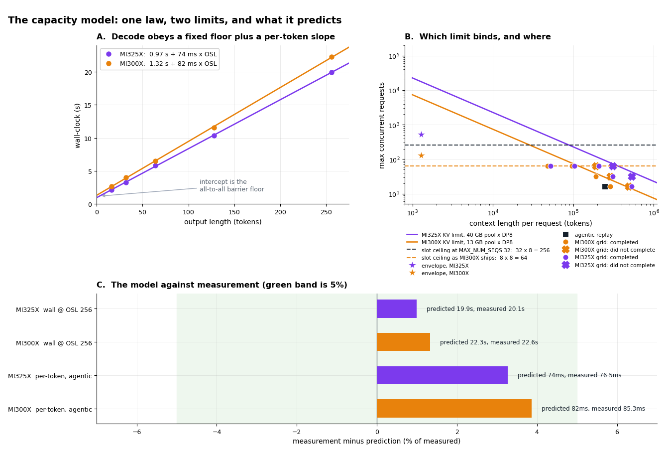
Figure 2. The decode-side capacity model in three panels

Figure 2. The decode-side capacity model in three panels. A, wall-clock against output length at concurrency 1. B, the KV-capacity and slot limits against context length, on log axes, with the measured operating points. C, each model prediction against its measurement, where the green band is 5%. Coincident grid points in panel B are nudged 4% apart along the context axis so both platforms stay legible.

From law to sizing calculator. One measured constant anchors everything: the KV cost per token is 14,098 bytes/token (the fp8 MLA latent), which matches the first-principles figure of 24 MLA layers x 576 elements/token x 1 byte to within 2%. With kv_tok in hand, the following three outputs follow:

Max concurrency at context L: N_max = KV_pool x DP / (kv_tok x L), capped in practice by the in-flight slot count and the measured knee. This is the output the KV pool governs directly, and it scales with the pool ratio of 3.1x. The multiplier is the data-parallel degree, 8, and not the 16 GPUs of a pool, because the MLA latent is replicated rather than tensor-sharded: both GPUs of a TP2 pair hold the same latent, so a pair contributes one pool’s worth of capacity and not two. The decode engines report this directly at startup. Each MI300X GPU allocates 916,875 KV tokens and each MI325X GPU 2,836,158, so a single GPU covers a full-length sequence on either platform, which it could not if the latent were split across the pair. Those counts also re-derive kv_tok from the other direction: 40 GB over 2,836,158 tokens is 14,104 bytes per token, against the 14,098 above. At 200K the formula gives 113 concurrent sequences on MI325X and 37 on MI300X.
Meets the latency SLA? wall = C0 + k · OSL; the maximum servable OSL at a latency budget T is (T − C0) / k.
Context ceiling: not a KV-capacity result for a single request. The per-GPU counts above are larger than either platform’s configured max_model_len, so the ceiling is the setting, and a recall ladder passes at every rung up to it on both.

Consider a worked example: serve 200K-context sessions, 32 concurrent, with 256-token replies. The following table walks the calculation through on both platforms:

Step	MI325X	MI300X
Context ceiling (measured and configured)	900K validated, `max_model_len` 1,000,000 ✓	900K validated, `max_model_len` 900,000 ✓
wall @ OSL 256	`0.97 + 0.074·256` = 19.9 s	`1.32 + 0.082·256` = 22.3 s
`N_max` @ 200K	113	37
In-flight slots	32 x 8 = 256	8 x 8 = 64
Meets 32 concurrent?	✓ (3.5x headroom on KV)	✓ (1.2x headroom on KV)

The latency output is validated, within 1.5% of measurement and independently reproduced by the agentic replay, as panel C of Figure 2 shows. The N_max output can be tested the same way, by walking context against concurrency until the serve stops completing requests. Each cell below is a wave of requests at a fixed input length, 64 output tokens, and ignore_eos. Table 2 sets the prediction against the outcome:

Context	MI300X `N_max`	MI300X highest served	MI300X lowest failed	MI325X `N_max`	MI325X highest served	MI325X lowest failed
50K	147	64	none reached	454	64	none reached
100K	73	64	none reached	227	64	none reached
200K	37	32	64	113	64	none reached
300K	24	16	32	76	32	64 (stall)
512K	14	none	16	44	16	32 (stall)

Table 2. The capacity grid against the concurrency N_max predicts. Each cell is a wave at a fixed input length with 64 output tokens. Where no failure is listed, concurrency 64 was the highest tested and the predicted limit sits far above it.

On MI300X every boundary the grid reached falls where N_max says it should: 37 predicted at 200K, with 32 completing and 64 not; 24 at 300K, with 16 completing and 32 not; and 14 at 512K, below even the lowest concurrency tested, which is why nothing completes there. Four of four completing cells sit under the KV limit and three of three failures sit above it, which is the prediction being right in both directions rather than merely not being contradicted. The two MI325X cells marked stall are the exceptions. Both fail well inside the limit, at 64 against a predicted 76 and 32 against 44, and both logged idle GPUs with no request completing, which is the signature of a stall rather than of a pool running out. They are reported as measured and are not explained by this model.

N_max is therefore a bound to size against and not merely an upper bound to quote. It remains a decode-side bound: it says what the KV pool admits, and says nothing about how long the prefill pool takes to fill it. Those waits are real and they are long. Serving 200K at concurrency 32 on MI300X keeps every request inside the KV budget and still takes 31 minutes of wall-clock, because two prefill nodes have 6.4M tokens to get through.

Why there is no matching prefill law here. The obvious thing to want is a second formula predicting time to first token from context length and concurrency, and the grid has 21 cells to fit it on. The fits are not good enough to publish next to a law that holds to 1.5%. A fixed ingest rate, meaning first-token time proportional to the prompt tokens a wave puts in front of the pool, explains about two thirds of the variance and misses individual cells by up to 58%. Allowing a request’s own prefill and its queue wait to carry separate coefficients does better on one platform and worse on the other. The best form tried, a power law in context and concurrency with exponents shared across both platforms, still averages 14% error and reaches 45%. Prefill time on a 2P2D shape depends on how a wave packs into the engine’s prefill chunks, which none of these forms represent, so the honest position is that capacity is modeled here and first-token latency is measured and reported instead. Figure 5 reports it.

Performance: Concurrency, Throughput, and Latency#

How far concurrency scales, what sets that ceiling, how throughput moves with request shape, and where the time goes in each half of the disaggregated serve.

The Concurrency Envelope#

Every request in this sweep has an input sequence length (ISL) of 1024 tokens and an output sequence length (OSL) of 256 tokens, with ignore_eos set so each one emits exactly 256. Concurrency is then swept from 1 to 512, watching for the point where wall-clock breaks off its single-request floor. Figure 3 plots both halves of that question:

Figure 3. Concurrency envelope

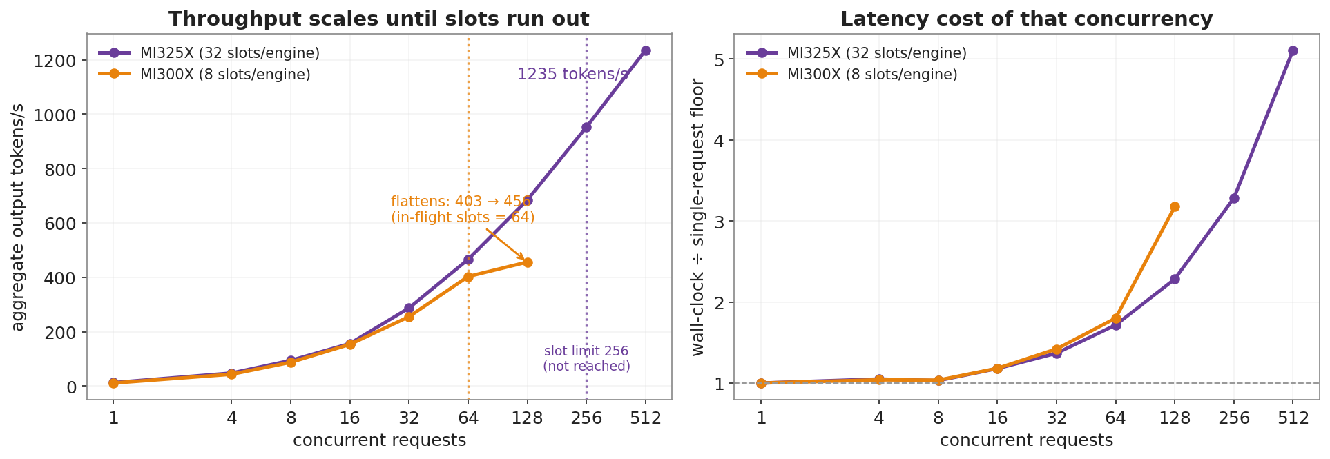
Figure 3. The concurrency envelope, both platforms. Left, aggregate output throughput against concurrency. Right, wall-clock as a multiple of the single-request floor, which is 20.1 s on MI325X and 22.6 s on MI300X.

MI325X rides that floor across the whole range tested: 512 times the load costs 5.1x the wall-clock while aggregate output throughput rises 96x, to 1235 tokens/s, with no plateau reached, so its ceiling lies beyond concurrency 512 and was not located here. MI300X reaches its limit at about concurrency 64, and the signature is unambiguous: throughput flattens, 403 to 456 tokens/s for a doubling of concurrency, while wall-clock climbs from 1.8x to 3.2x the floor. Concurrency is close to free while a request finds a free in-flight slot, and the curve bends once it has to queue.

One measurement note on that sweep. The harness also reports a completed-request count, and that counter is unreliable: it scores completeness from streamed events, which coalesce under load, so it marks finished requests incomplete. An instrumented rerun returned finish_reason = length for every request at concurrency 1, 16 and 32, with no exceptions and end-to-end times of 20 to 27 seconds against an 1800-second timeout. Completion is therefore 100% through that range, and because the throughput figures derive from the same token counter, they are lower bounds rather than overstatements.

Where the time goes inside those numbers. Aggregate throughput says what the pool delivers; it does not say what a caller waits. Replaying the same ISL 1024 and OSL 256 shape with per-request instrumentation on MI325X separates the two halves of that wait, time to first token (TTFT) and time per output token (TPOT). Table 3 splits the wait:

con	TTFT p50	TTFT p99	TPOT	out tokens/s	total tokens/s
4	1.2 s	1.2 s	74.9 ms	51	257
8	2.2 s	2.2 s	72.5 ms	89	447
16	3.2 s	3.2 s	77.3 ms	134	670
32	6.4 s	6.4 s	80.8 ms	278	1,388
64	7.6 s	11.1 s	94.1 ms	454	2,272
128	10.9 s	19.9 s	101.2 ms	675	3,374

Table 3. Latency and throughput inside the envelope, MI325X, same request shape as Figure 3. TPOT is derived as end-to-end time minus TTFT, divided by the 255 tokens after the first. Total tokens per second counts input and output together, at 1280 tokens per request.

Two things in Table 3 are worth drawing out. TPOT at concurrency 4 is 74.9 ms against the 74.0 ms slope fitted from the controlled output-length sweep, so the capacity model reappears in an independent measurement. And concurrency is not free in the way aggregate throughput alone suggests: from concurrency 4 to 128 the pool delivers 13x more output tokens per second, but TPOT inflates 1.35x and TTFT climbs from 1.2 to 10.9 seconds at the median and to 19.9 seconds at p99. That is prefill queueing ahead of the first token, not slower decoding. Because total tokens per second counts the input too, it runs about 5x the output figure, and it is the number to quote for a prefill-heavy deployment. These per-request timings exist only for MI325X, since no MI300X run at this shape recorded them, so the cross-platform comparison stays on Figure 3 where both platforms have matched data.

What Sets the Knee#

The gap between the two platforms invites a KV-pool explanation, but the arithmetic does not support one at these lengths. At ISL 1024 and OSL 256 a sequence holds roughly 1280 tokens, or about 18 MB of key-value cache, so the decode pool could in principle hold tens of thousands of them: about 35,000 concurrent sequences on MI325X and about 11,500 on MI300X. The binding constraint is instead the number of in-flight sequence slots: MAX_NUM_SEQS per engine multiplied by the eight data-parallel lanes:

Platform	`MAX_NUM_SEQS`	in-flight slots	observed behaviour
MI325X	32	32 x 8 = 256	no plateau within the range tested
MI300X	8	8 x 8 = 64	plateaus at 64

That the MI300X plateau lands exactly on its slot count is suggestive but, on its own, only a coincidence. So it was tested directly: hold the hardware, the 13 GB KV pool and the request shape fixed, raise MAX_NUM_SEQS from 8 to 32, and see whether the knee moves. It does, as Table 4 shows.

con	`MAX_NUM_SEQS` = 8	`MAX_NUM_SEQS` = 32
32	255 tokens/s	245 tokens/s
64	403 (knee)	386 tokens/s
128	456 (plateau, +13%)	586 (+52%, still climbing)

Table 4. The same MI300X pool at two slot ceilings, ISL 1024 and OSL 256, with every request completing in both runs.

Table 4 reports that intervention. At MAX_NUM_SEQS = 8 throughput gains only 13% for the doubling from concurrency 64 to 128, the signature of a queue. At 32 the plateau is gone: the same doubling gains 52%, reaching 586 tokens/s and still rising at the concurrency 128 cap, which puts the next knee near 32 x 8 = 256. The knee is therefore set by in-flight slots and is a configuration choice, not a property of the silicon. The larger setting is also marginally slower at low concurrency, 245 against 255 tokens/s at concurrency 32, so the slot ceiling is a throughput-versus-latency trade rather than a free win.

This makes the limiter a measured result and no longer an inference, and it changes the practical advice: MI300X’s concurrency 64 plateau is not where the hardware gives up, it is where the recipe was set. Raising the ceiling recovers 28% more throughput at concurrency 128 on the same pool.

The KV pool is still the reason the shipped recipes differ: 13 GB cannot safely admit 32 concurrent long-context sequences, so the conservative MI300X default is 8. The distinction matters because it tells you which knob to reach for. At short context the knob is MAX_NUM_SEQS, which costs nothing to change. At long context the pool itself binds, and that is where hardware is the answer.

Throughput Across Request Shapes#

A throughput-class matrix rounds out the picture at larger request shapes than the envelope’s fixed 1024 and 256. Table 5 lists three synthetic classes, a latency-floor shape, a throughput-peak shape, and a long-context shape, measured on both platforms. Every request completed in all six runs:

class	ISL and OSL	con	MI300X out tokens/s	MI300X total tokens/s	MI325X out tokens/s	MI325X total tokens/s
latency-floor	128/32	16	146	719	175	854
throughput-peak	1024/1024	64	570	1026	368	981
long-context	32K/512	32	87	4318	40	4420

Table 5. Throughput classes on both platforms, at identical request shapes, with every request completing.

The long-context shape is the striking one. Dominated by the 32K-token prefill ingested per request, it reaches 4318 total tokens/s on MI300X and 4420 on MI325X, far above either platform’s output-token rate, and that is what a prefill-heavy workload looks like measured end to end. The two platforms also do not order consistently across the three classes. MI325X leads at the latency-floor shape, 175 against 146 output tokens/s, and is marginally ahead on long-context total throughput. MI300X leads clearly at the throughput-peak shape, 570 against 368 output tokens/s at concurrency 64. No single platform ranking survives a change of request shape, which is why this post reports an envelope and a class matrix instead of one headline number.

Figure 4 draws both of those axes together. In panel A, aggregate throughput rises 13x between concurrency 4 and 128 while the per-token cost rises with it, from 74.9 to 101.2 ms, and the shading marks where the first-token tail leaves the median behind: 7.6 s against 11.1 s at concurrency 64, and 10.9 s against 19.9 s at 128. That divergence is the part a median-only report hides. Panel B shows why the metric has to match the workload. MI300X is 1.5x ahead on the throughput-peak shape and 2.2x ahead on long-context output, yet those same long-context runs are within 2% of each other on total throughput, at 4,318 against 4,420.

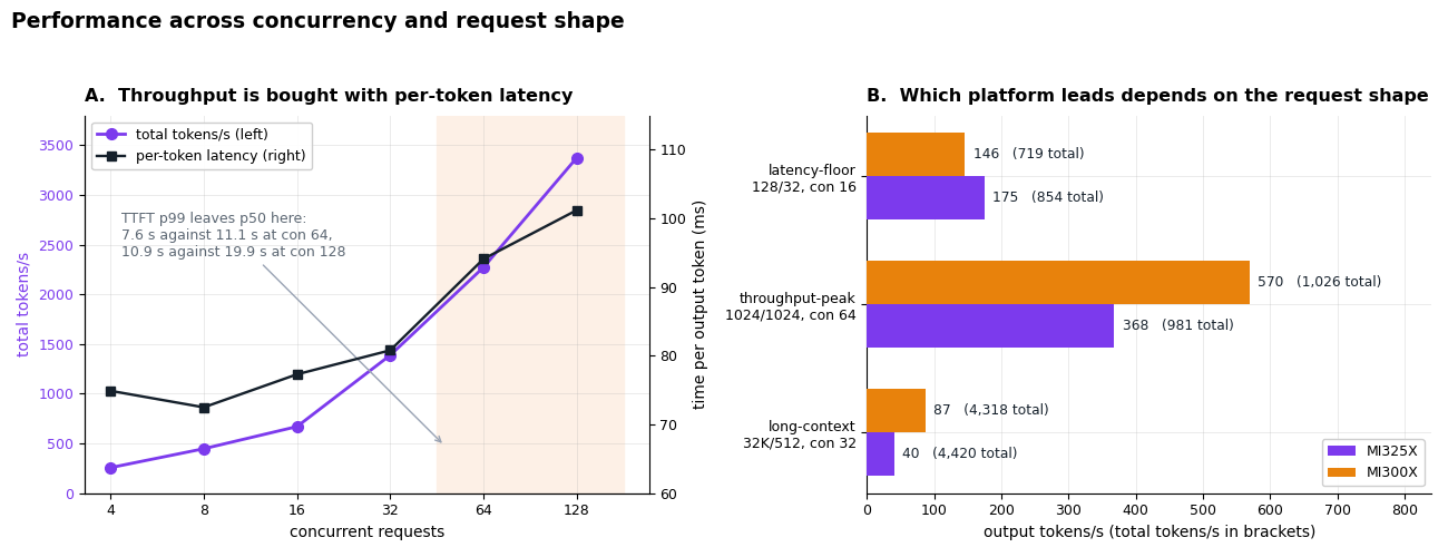
Figure 4. Performance across concurrency and request shape

Figure 4. The two performance axes side by side. Panel A is the interior of the MI325X envelope from Table 3, with the shaded region marking where the time-to-first-token tail separates from the median. Panel B is Table 5 drawn to scale, where bar length is output tokens per second and the bracketed figure is total tokens per second.

Latency: TTFT and TPOT in a Disaggregated Serve#

Disaggregation splits latency across two machines, so the two halves are reported separately. TTFT is prefill compute plus the MoRIIO KV-cache transfer from prefill to decode, the disaggregation tax. Inter-token latency (ITL), equivalently time per output token (TPOT), is steady-state decode on the decode pool alone.

Both halves come from the small agentic profile replayed at concurrency 1, which streams token by token and so measures them directly, on the same instrument for both platforms. MI325X reaches first token in 1.17 s at a median input of 1,792 tokens and then sustains 76.5 ms per token. MI300X takes 1.65 s at 2,080 tokens and 85.3 ms. Inputs come from a trace corpus rather than a fixed length, so the median input differs between the two and the TTFT figures should be read with that in mind; the per-token figure is unaffected, because it measures steady-state decode after prefill completes. These are the concurrency-1 rows of Table 7, reported here because the latency question belongs to this section, and the sample behind the MI300X figure is 13 completed requests.

Taking them from the replay instead of from the fitted constants matters: the floor C0 and slope k come from the output-length sweep, so quoting them back as measured TTFT and TPOT would make the later cross-check circular. A separate instrument keeps that comparison, where ITL is set against k in the agentic section, independent.

Those figures are the short-context case. The capacity grid behind Table 2 measured the same two quantities at every cell it ran, and at long context they look different. Figure 5 reports them.

Read panel A for the absolute size of the wait, which is what it measures reliably. First-token latency runs from about a minute at 50K and concurrency 16 to 33 minutes for MI325X at 512K, a cell Table 2 records as served. Do not read it for the ratio between the curves. MI325X sits below MI300X at every shared cell, but the MI300X cells all come from a single allocation, and a second MI300X allocation measured the same 200K concurrency-16 shape 2.1x faster. Within this campaign the platforms differ by 1.14x at concurrency 1 and 2.34x at concurrency 16 on the same probes, so the gap under load sits somewhere between roughly 1.1x and 2.3x, and this data does not place it. Panel B carries a cleaner result: aggregate throughput does not track context at all, and a tenfold change in context length leaves every run inside the same 1,800 to 4,700 tokens per second band, which is what a prefill-bound stage looks like from the outside. No line is fitted through panel A because none is good enough. First-token latency does correlate with the prompt work a wave puts in front of the prefill pool, at a Pearson correlation of 0.83 on MI300X and 0.78 on MI325X, but a fixed-rate model misses individual cells by as much as 58%.

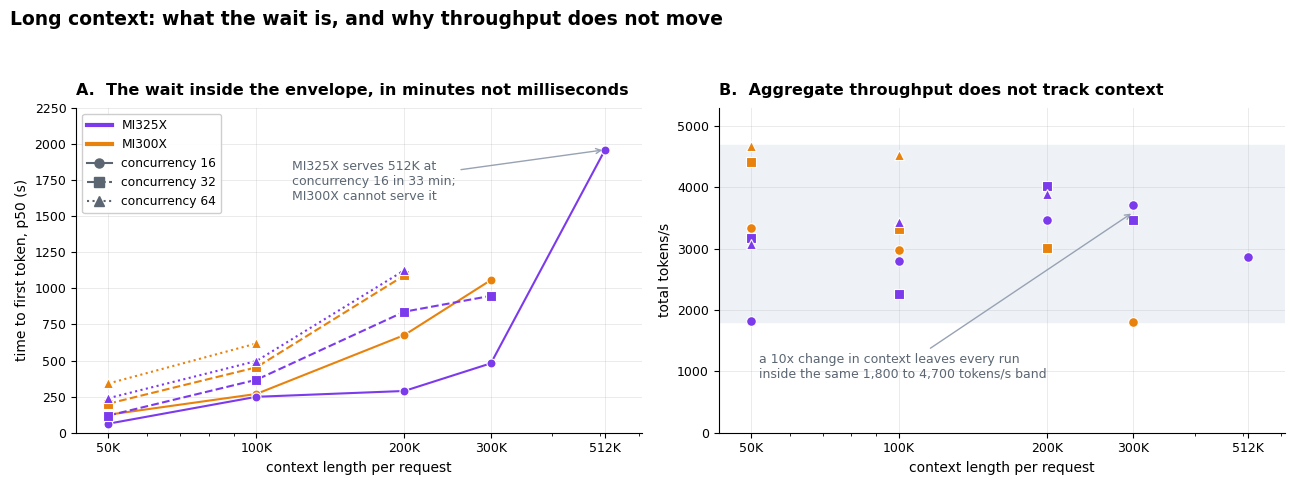
Figure 5. Long-context latency and throughput

Figure 5. The 21 capacity-grid cells, reporting what Table 2 reduced to a served-or-failed verdict. Panel A, first-token latency against context. Panel B, aggregate throughput against the same axis. No line is fitted through panel A; the scaling is shown rather than modeled.

The practical reading is that capacity and latency are separate questions. A cell can sit inside the KV bound, complete every request, and still make a user wait half an hour for the first token.

Long Context: How Far One Request Can Go#

Concurrency is one axis; context length is the other, and it is bounded by different physics. The third limit is how much context a single request can reach. Recall itself is covered in the accuracy section. What this section adds is the shape of the curve and where each platform stops. Both platforms recall at every rung to 900K, and on both the stopping point is the configured max_model_len rather than anything physical: 1,000,000 on MI325X, 900,000 on MI300X. The KV pool is not what stops either one. The MI300X decode pool reports 916,875 tokens per GPU, which is more than the 900,000 it was configured to accept, so the last rung tested is the largest request the serve was allowed to admit and not the largest it could hold.

Figure 6 plots the curve. Both platforms scale close to linearly, which is the signature of a prefill-dominated single request, and the MI300X curve sits above the MI325X one by a roughly constant factor. That gap is prefill and not decode, so it is not the decode graph-capture difference in the configuration table: prefill runs eager with no capture on both platforms, and a request on this ladder decodes about 19 tokens, which puts the entire per-token difference at 0.15 s of the 285 s separating the two 900K rungs. What is left is memory bandwidth and fabric, which this measurement does not separate.

Figure 6. Memory frontier

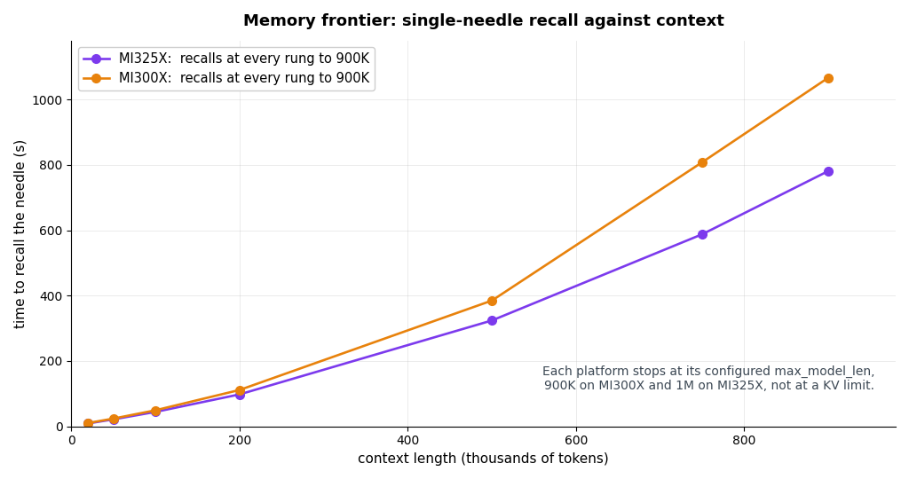
Figure 6. Needle-recall time against context length, both platforms, to 900K tokens. The MI300X 750K and 900K rungs come from a later run that measured about 12% slower throughout.

Agentic Evaluation with AgentX#

Synthetic sweeps use fixed shapes; real traffic does not. To test whether the capacity model survives real load, multi-turn agentic session traces are replayed with the AgentX suite, merged in ROCm/MAD and wrapping the aiperf inferencex-agentx-mvp scenario. Each workload builds or downloads a session corpus and replays it against the live router, with sessions arriving on independent lanes so that turn boundaries, think-time gaps, and prefix reuse survive into the serve.

Two kinds of corpus are used, and they carry different guarantees. The small and conformance corpora are synthesized against a declared profile and can therefore be verified against it: a pre-gate compares the generated corpus with its own profile across 13 axes, four distribution metrics at three percentiles plus the median cache-hit rate, and all three passed 13 of 13 before any number was taken from them. The inferencex_256k corpus is a recorded InferenceX trace replayed as captured, so the generator pre-gate does not apply to it.

Three regimes are probed:

small (input 2 to 7K), at concurrency 1 for the clean cross-check against the single-stream slope k, and at concurrency 16 to confirm ITL inflates as the envelope predicts and not arbitrarily.
inferencex_256k, a recorded InferenceX trace filtered to 200K input or less: realistic long-context traffic with heavy prefix-cache reuse.
conformance_256k and conformance_512k, synthesized near-ceiling and beyond-ceiling stress. Only MI325X runs the 512K profile; it was not attempted on MI300X.

What each corpus contains is what makes the results readable, and Table 6 lays it out:

Profile	Sessions	Turns	Input p50 / p99	Output p50 / p99	Cache reuse	Platforms
`small`	200	479	1,849 / 7,000	129 / 468	85%	both
`inferencex_256k`	984	10,035	recorded, filtered to 200K	recorded	85 to 99%	MI300X
`conformance_256k`	200	1,778	74,140 / 245,000	306 / 16,193	88%	both
`conformance_512k`	300	6,917	61,490 / 520,000	176 / 7,151	88%	MI325X

Table 6. What each replay corpus contains. Sessions and turns are the whole corpus as laid onto the replay lanes, and the token counts are measured on the generated corpus against the distribution its own profile declares. The recorded InferenceX corpus declares no target distribution, so its cells report what the trace carries.

Three details in Table 6 shape how the results read. Turn depth is what makes this agentic traffic rather than a set of long single prompts: conformance_256k reaches 103 turns at p99 and conformance_512k reaches 144, against 6 for the short corpus. The output tails are long and heavily skewed, a p50 of 306 tokens against a p99 of 16,193 on conformance_256k, which is why output throughput on these profiles is set by the traces and not by the serve. And two sessions of conformance_512k sit above the 524,288-token context limit and are dropped at load, so 298 sessions and 6,663 turns of it actually reach the lanes.

Concurrency 1 is the cross-check, and it lands: real-trace ITL reproduces the slope fitted from the controlled output-length sweep on both platforms, 76.5 ms against a fitted 74 ms on MI325X and 85.3 ms against 82 ms on MI300X, agreeing to within 3% and 5%. A per-token cost extracted from a synthetic sweep reappearing under real multi-turn traffic is what makes the capacity model a mechanism and not a fit artifact.

With that anchor in place, the replay runs span input p99 from roughly 6K to 414K. Figure 7 puts them all on one pair of axes. Time to first token tracks input length across two orders of magnitude, which is the prefill-bound signature, and inter-token latency holds near the fitted slope at concurrency 1 before rising to roughly 0.5 to 0.7 s at 160K to 244K and 1.14 s at 414K, because every decode step attends over a larger cache.

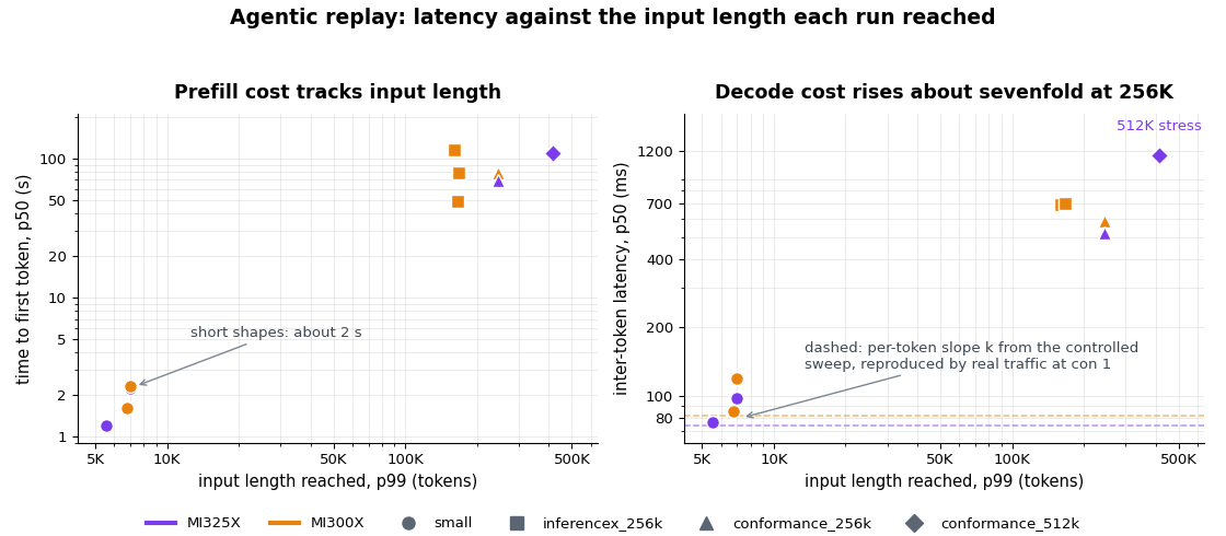
Figure 7. Agentic replay latency against input length

Figure 7. Latency against the input length each replay run actually reached, every run on one pair of axes, both scales logarithmic. Color is platform, marker is corpus, and the dashed lines are the fitted per-token slope k.

Table 7 gives the per-run figures behind that plot:

Platform	Profile	con	requests	input p99	TTFT p50	ITL p50	active tokens/s	cache hit
MI325X	`small`	1	64	5,553	1.2 s	76.5 ms	166	42%
MI300X	`small`	1	13	6,772	1.6 s	85.3 ms	188	39%
MI325X	`small`	16	808	7,024	2.2 s	97.7 ms	2,139	36%
MI300X	`small`	16	690	7,024	2.3 s	118.4 ms	1,812	37%
MI300X	`inferencex_256k`	2	1	160,574	115.2 s	693 ms	339	99%
MI300X	`inferencex_256k`	4	6	166,418	49.3 s	710 ms	543	86%
MI300X	`inferencex_256k`	8	16	166,589	78.6 s	699 ms	1,609	96%
MI300X	`conformance_256k`	16	30	244,090	79.1 s	589 ms	3,010	55%
MI325X	`conformance_256k`	16	25	244,239	69.9 s	523 ms	2,448	56%
MI325X	`conformance_512k`	16	35	414,631	109.3 s	1,141 ms	3,561	35%

Table 7. Every replay run in full. The requests column is how many turns completed inside the 900 s measurement window. Throughput is active total tokens per second, which excludes the inter-turn think-time gaps the traces carry.

Four cautions apply when reading Table 7. The request counts are small on the long-context rows because one 244K-token turn costs roughly 80 s of prefill before it emits anything, so the two inferencex_256k rows at concurrency 2 and 4, which completed 1 and 6 requests, are individual observations rather than percentiles. The like-for-like cross-platform comparison is the conformance_256k pair, which replays the same corpus at concurrency 16 and reaches a matched input p99 near 244K; read it at the percentile and not the mean, because real traces carry a length distribution and the two runs drew different means. Throughput is not comparable between rows with different output-length distributions or cache-hit rates. And the non-zero error counts in the raw artifacts are not wire errors: they are grace-period session cancellations at the measurement cutoff, where a very large session is truncated rather than failed, plus two tail traces above 524,288 tokens that the context gate dropped by design. Nothing wedged in any of these runs, and every run completed with no in-window wire errors on either platform.

Three things follow from the replay runs:

Under load, ITL inflates by the predicted factor. At concurrency 16 the short corpus reaches 97.7 ms on MI325X and 118.4 ms on MI300X, 1.28x and 1.39x their concurrency-1 values: the same k scaled by decode-batch contention, with MI325X inflating less on its larger headroom.
Long-context agentic load runs clean. Multi-turn traffic at a 244K input p99 on both platforms, and 414K on MI325X, made continuous progress with no in-window wire errors, so nothing about the synthetic long-context probes carried over into realistic replay.
Long-context agentic traffic is prefill-bound. TTFT dominates while each turn emits few tokens, so output tokens per second is low by design and is not a throughput ceiling.

Lessons Learned#

Four lessons generalize beyond this model, and every one of them is about measurement rather than serving.

Verify the instrument before characterizing the platform. The concurrency envelope’s harness reports a completed-request count, and under load that counter read as low as 37% on runs where the tokens demonstrably arrived, because it infers completeness from streamed events that coalesce under load. Taken at face value it supports a confident and wrong conclusion about the platform. The check that caught it was arithmetic: aggregate throughput times wall-clock came within 90 to 100% of the forced output length at every rung, and a run cannot deliver 97% of its expected tokens while 44% of its requests fail. An instrumented rerun then confirmed finish_reason = length on every request.

A probe’s construction can manufacture a model failure. The single-needle ladder originally reported intermittent recall at 100K. The cause was the haystack: filler built by repeating one sentence is adversarial for linear attention and produces misses even at concurrency 1. The same rung with non-repetitive filler recalls every time. Any NIAH result against a hybrid-attention model should state how its haystack was built.

A failure that does not survive a fresh serve is not a platform property. Two of the sharpest results here were retracted by rerunning them. A 750K recall attempt wedged on every try, with decode GPUs pinned and no tokens emitted, and 200K at concurrency 32 took the prefill API-server processes down while decode KV usage sat at 6%. Both looked like hard limits, and both were written up as such. On clean serves, both the 750K and 900K rungs pass, and 28 of 32 requests complete at 200K and concurrency 32. Neither diagnosis was wrong about what happened; both were wrong about what it meant. A failure observed once on one serve is a fact about that serve until a second serve reproduces it, and the cost of skipping that second serve is a published claim that has to be withdrawn.

Cite from preserved artifacts, not from reports. An earlier summary of the recall ladder carried times that matched no surviving run, and they were quoted for weeks before anyone tried to locate the output. The fix is procedural: publish from an artifact that ships, and treat a number whose artifact cannot be found as unmeasured.

Reproducibility#

The recipe is packaged in ROCm/MAD PR #241: a Dockerfile with all component pins baked in, four-node launch scripts (workers, then masters, then router), and the accuracy, performance, and NIAH probes, all driven by environment variables. Bring-up order is workers before masters before router; the decode pool uses mori_low_latency with FULL_AND_PIECEWISE (MI325X) or PIECEWISE (MI300X), and the prefill pool uses mori_high_throughput with eager execution. The MoE path is selected with AITER_SITUV2_A8W4=1, and the KV write-race barrier with K3_WRITE_READBACK=1.

The synthetic measurements in this post can be regenerated instead of taken on trust, because the probes behind them ship in that same pull request: the concurrency envelope, the output-length sweep, the performance classes, the single-needle NIAH ladder, and the distinct-needle concurrency gate. Each takes the router URL from the environment and the request shape from the command line, so reproducing a given table means running the matching probe against a serve brought up with the recipe above. The agentic replay comes from a different open-source location, not from a packaged probe: the AgentX suite is merged in ROCm/MAD under scripts/common/agentx, and the four profiles reported here ship with it, so those runs are reproducible from the profile definitions and the recorded trace corpus they reference. The raw measurement artifacts behind the tables are not published with this post.

An Operational Note on Draining High-Concurrency Waves#

One behaviour is worth passing on because it costs time to rediscover. When a high-concurrency wave is killed from the client side instead of allowed to drain, the MoRI-IO fabric on this 2P2D deployment can be left in a state where it no longer completes concurrent KV transfers, while single-request traffic keeps working normally. The signature is specific: concurrency 1 passes, every higher rung reports ok=0, the GPUs sit near 0% with a silent router, and the prefill side logs MoRI-IO Deferred write task ... expired after 60.0s (remote blocks never arrived). It reproduced three times, including on an otherwise quiet serve, and it appeared only after a concurrency-512 wave had to be hard-killed.

The practical consequences are small but worth knowing. Relaunch the serve after any hard-killed wave instead of trusting the next sweep, because a serve that reports ready at concurrency 1 can still be degraded for concurrent work. Cap concurrency ladders at the rung you actually need, which is why the MI300X envelope here stops at 128. And when a sweep reports a sudden floor of ok=0 above concurrency 1, suspect fabric state from a previous run before concluding anything about capacity: the same recipe sustained concurrency 32 and 64 cleanly at a larger request shape immediately beforehand.

Summary#

This post brings a 1.4 TiB MXFP4 mixture-of-experts model to AMD Instinct and turns “can it run” into “here is exactly what it costs.” The model does not fit one node, so the 896 experts are sharded EP16 across a 2P2D disaggregated deployment and the non-shardable attention is split with TP2 x DP8, the only layout that fits both 192 GB and 256 GB. MXFP4 does not run natively on gfx942, so the int4-SiTU path that the hardware actually accelerates is used. The hybrid KDA and MLA architecture hid two concurrency bugs; both were found and fixed, and distinct-needle recall under concurrency is 57 of 57 on both platforms.

The payoff is a decode-side capacity model you can compute before you deploy. Per-token decode speed is comparable across MI300X and MI325X, at 74 against 82 ms/token, so compute is not the axis that separates them. What separates them is capacity, and the useful result is that three different limits bind in three different regimes. Short-context concurrency is bounded by in-flight sequence slots, so MI300X plateaus at exactly concurrency 64 while MI325X rides the floor to concurrency 512 and 1235 tokens/s. That plateau is a configuration setting, not a hardware limit, and raising MAX_NUM_SEQS on MI300X moves the knee and buys 28% more throughput at concurrency 128. Long-context concurrency is bounded instead by the KV pool, a 3.1x gap that the per-token arithmetic predicts exactly. The context ceiling is 900K on both platforms, set by the configured max_model_len rather than by KV bytes, which the measured per-GPU KV pool confirms on each.

None of that would mean much if it only held for fixed request shapes, so the last check is real traffic: multi-turn agentic sessions, over a hundred turns deep in places, replayed to a 244K input p99 on both platforms and 414K on MI325X. They run clean, the per-token cost reappears within 3 to 5% of the fitted slope, and inter-token latency grows with context the way the model says it should, from about 77 ms at short shapes to 590 ms at 256K and 1141 ms at 512K.

So the deployment question, which GPU, how many nodes, how much context, how much concurrency, becomes a calculation instead of a guess, and it also tells you when the answer is a configuration change instead of a purchase. Work that stays inside 200K context at concurrency 32, or 300K at 16, is well served by MI300X, and the slot ceiling at short context is a setting to raise there, not a reason to buy. A step beyond that in either direction is where MI325X’s larger KV pool is the answer, because that is the one limit no configuration change can move.

This post is part of the AMD Disaggregated Inference (DI) Blog Series, which follows open frontier models from a single-node demo through to multi-node serving on AMD Instinct GPUs, one model at a time. If this deployment is useful to you, the first post in the series, Scaling GLM-5.1-FP8 to 64 MI300X GPUs, applies the same disaggregated wide expert-parallel approach to a different model, and more posts are to follow.

Additional Resources#

The following posts, code, pull requests, and issues back the work in this post:

AMD ROCm Blog: DI Series, Scaling GLM-5.1-FP8 to 64 MI300X GPUs: the first post in this series, covering the sibling disaggregated wide-EP study. The following code, pull requests, and issues back the work in this post:
ROCm/MAD PR #241: the Kimi-K3 disaggregated recipe (this work).
AgentX: the agentic-replay benchmark suite used for the evaluation in this post, merged and open source in ROCm/MAD. The profiles directory contains the four profiles reported here, small, inferencex_256k, conformance_256k and conformance_512k, so the replay shapes can be read directly instead of described. Contributed by ROCm/MAD PR #213, which wraps the aiperf inferencex-agentx-mvp harness.
vLLM MoRIIO RDMA read-after-write barrier: raviguptaamd/vllm@206fffe.
vLLM issue #35219: mamba and KDA recycled-block zeroing.
ROCm/aiter PR #4471: SiTUv2 activation in the int4 stage-1 epilogue.
ROCm/mori: MoRI-EP all-to-all and the MoRIIO connector.

The following papers and specifications describe the techniques and formats this deployment relies on:

Multi-head Latent Attention: DeepSeek-V2 and DeepSeek-V3, arXiv:2405.04434 (the MLA KV compression Kimi-K3 uses).
Gated DeltaNet: Yang et al., arXiv:2412.06464 (the fixed-state recurrent class of the KDA layers).
DistServe: Zhong et al., OSDI 2024, arXiv:2401.09670 (the prefill-decode disaggregation principle).
Wide expert parallelism: DeepSeek-V3, arXiv:2412.19437 (large-EP dispatch and combine all-to-all).
PagedAttention and vLLM: Kwon et al., SOSP 2023, arXiv:2309.06180 (the serving engine and KV pool).
OCP Microscaling Formats (MX) Specification v1.0: the MXFP4 block format the weights ship in.
Hugging Face model card: moonshotai/Kimi-K3.

System Configuration#

The following sections list the hardware, serving knobs, and software pins used for every measurement in this post.

Hardware#

The following table lists the hardware used on each platform:

Component	MI325X	MI300X
Accelerator	AMD Instinct MI325X (gfx942)	AMD Instinct MI300X (gfx942)
HBM per GPU	256 GB	192 GB HBM3
GPUs per pool	16 (2 nodes x 8)	16 (2 nodes x 8)
Fabric	Broadcom BCM57608 “Thor2” 400G RoCE v2 (bnxt_re), 8 rails	NVIDIA ConnectX-7 (mlx5), RoCE and InfiniBand
Intra-node	xGMI	xGMI

Serving Configuration (Per Platform)#

Both platforms run the same image and the same recipe, but several serving knobs differ, and in every case the reason is the memory budget, not a tuning preference. The following table lists the knobs that differ and why:

Knob	MI325X	MI300X	Why it differs
Prefill CUDA graph	eager, no capture	eager, no capture	Same on both. Prefill is compute-bound and bursty, so graph capture buys nothing.
Decode CUDA graph	`FULL_AND_PIECEWISE`	`PIECEWISE`	Memory. Capturing the full graph family alongside weights, KV pool and communication heap does not fit in 192 GB: the MI300X recipe caps its capture list at batch size 32 because the 40, 48, 56 and 64 entries ran out of memory during capture. With 256 GB the whole family captures.
Prefill all-to-all	`mori_high_throughput`	`mori_high_throughput`	Same on both. Throughput-optimized dispatch and combine for the prompt burst.
Decode all-to-all	`mori_low_latency`	`mori_low_latency`	Same on both. Latency-optimized for the token stream.
KV pool	40 GB	13 GB	Whatever HBM remains after 137.5 GiB per GPU of weights, the MoRI heap, and graph capture.
`max_model_len`	1,000,000	900,000	Trimmed on MI300X so the KV reserve fits the smaller pool.
MoRI shared heap	16 GiB	6 to 8 GiB	Reduced on MI300X to leave room for weights and graph capture; the later allocation ran 6 GiB.

The decode CUDA-graph split is the most consequential of these. It is not a preference: the full graph family is affordable on 256 GB and is not on 192 GB. That is the same memory arithmetic that opens this post, reappearing at the level of a single launch flag. Graph capture also competes directly with the KV pool, so the 40 GB against 13 GB difference in the table above and the capture mode beside it are two readings of one budget.

Software#

The following table lists the software pins used for every measurement in this post:

Component	Pin
vLLM	`raviguptaamd/vllm@206fffe` (branch `v4-disagg-situ-restore-mambafix`, off `184535a92`)
MoRI	`624002c897a3` (built from source)
AITER and FlyDSL	`0.1.19` and `0.2.4` (int4-SiTU, SiTUv2 a8w4)
Base image	`rocm/vllm-dev:ci_base-dedbf6be` (ROCm 7.2, cp312)
Router	vllm-router (PD-disaggregation discovery)
Model	`moonshotai/Kimi-K3` (MXFP4, 96 safetensors shards, native max 1,048,576 tokens)

Disclaimers#

The information presented in this document is for informational purposes only and may contain technical inaccuracies, omissions, and typographical errors. The information contained herein is subject to change and may be rendered inaccurate for many reasons, including but not limited to product and roadmap changes, component and motherboard version changes, new model and/or product releases, product differences between differing manufacturers, software changes, BIOS flashes, firmware upgrades, or the like. Any computer system has risks of security vulnerabilities that cannot be completely prevented or mitigated. AMD assumes no obligation to update or otherwise correct or revise this information. However, AMD reserves the right to revise this information and to make changes from time to time to the content hereof without obligation of AMD to notify any person of such revisions or changes. THIS INFORMATION IS PROVIDED “AS IS.” AMD MAKES NO REPRESENTATIONS OR WARRANTIES WITH RESPECT TO THE CONTENTS HEREOF AND ASSUMES NO RESPONSIBILITY FOR ANY INACCURACIES, ERRORS, OR OMISSIONS THAT MAY APPEAR IN THIS INFORMATION. AMD SPECIFICALLY DISCLAIMS ANY IMPLIED WARRANTIES OF NON-INFRINGEMENT, MERCHANTABILITY, OR FITNESS FOR ANY PARTICULAR PURPOSE. IN NO EVENT WILL AMD BE LIABLE TO ANY PERSON FOR ANY RELIANCE, DIRECT, INDIRECT, SPECIAL, OR OTHER CONSEQUENTIAL DAMAGES ARISING FROM THE USE OF ANY INFORMATION CONTAINED HEREIN, EVEN IF AMD IS EXPRESSLY ADVISED OF THE POSSIBILITY OF SUCH DAMAGES. AMD, the AMD Arrow logo, ROCm, Instinct, and combinations thereof are trademarks of Advanced Micro Devices, Inc. Other product names used in this publication are for identification purposes only and may be trademarks of their respective companies. © 2026 Advanced Micro Devices, Inc. All rights reserved.

Third-party content is licensed to you directly by the third party that owns it and is not licensed to you by AMD. Benchmark results are preliminary and measured on AMD Instinct™ MI300X and MI325X (gfx942); actual performance may vary based on configuration, software versions, drivers, and optimizations.