Attention Decode on AMD MI450 GPUs: A Gluon Kernel Optimization Guide

July 27, 2026 by Pengzhan Zhao, Lixun Zhang, Lei Zhang (antiagainst).

14 min read. | 3480 total words.

Software tools & optimizations

AI/ML, Linear Algebra, Performance, Profiling, Optimization, Hardware, Compiler

HPC

Agentic AI applications are pushing LLM inference into a new regime. A request can now reach one million tokens from aggregated long prompts, tool calls, retrieval results, and multi-turn reasoning. During the text generation phase, each new token must attend to all previous tokens from the KV cache, so the kernel needs to repeatedly read past states from HBM. As a result, the performance bottleneck shifts from compute units to the memory system.

The AMD Instinct MI450 series GPU introduces a new set of hardware features for memory-sensitive AI workloads. This blog uses attention decode as a case study and discusses how to design a high-performance kernel on MI450. We will walk through core hardware features, explain how kernels can use these features, and showcase the performance of an optimized Gluon kernel, which achieves 85% of the peak HBM bandwidth on MI450 as an early result.

MI450 Hardware Overview

MI450 is a large step forward from the MI350 series for AI workloads. Compared with previous generations, MI450 provides more on-chip resources and larger HBM capacity with higher bandwidth. The following table summarizes the key spec changes between MI350 and MI450. A Workgroup Processor (WGP) is the hardware unit that runs a workgroup (named CU in earlier MI-series). In this model, one WGP contains four SIMD32 units, each with 32 lanes. Each SIMD32 has its own Vector General-Purpose Registers (VGPRs), which are used by the Vector ALU unit (VALU) and Wave Matrix Multiply-Accumulate unit (WMMA). All SIMD32 units in a WGP share the same Local Data Share (LDS) memory.

Specification	MI350 series	MI450 series
VGPRs per SIMD	512	1024
Max LDS per WGP	160 KB	320 KB
HBM capacity	288 GB	432 GB
HBM bandwidth	8.1 TB/s	19.6 TB/s

In addition to more on-chip resources, MI450 introduces a specialized hardware unit - TDM, to help move structured tensor data between global memory and LDS. With TDM, the kernel describes the target tensor to access using its memory address, shape, strides, and layout, then issues a bulk data transfer asynchronously. TDM helps accelerate memory access and also makes it easier to write pipelined kernels where compute and memory can be overlapped. This marks a significant change from MI350, where the kernel must issue many small vector loads to move data from global memory to LDS.

Features	MI350 series	MI450 series
Memory instruction	Global/Buffer load to LDS	TDM load to LDS
Load granularity	32/96/128-bit vector loads	Descriptor-based tensor tiles
Memory units per WGP	1	2

Moreover, MI450 further extends the workgroup model with workgroup clusters. A normal workgroup runs on one WGP, independently of other workgroups. A cluster lets several workgroups, each running on its own WGP, coordinate through hardware-supported cluster barriers. Workgroups that access the same data can use multicast loads to share data across WGPs. This gives kernels a way to express cooperation at a larger scope, without falling back to a separate kernel launch or using global memory for synchronization.

The figure below shows a kernel programmer’s view of the whole MI450 GPU hierarchy.

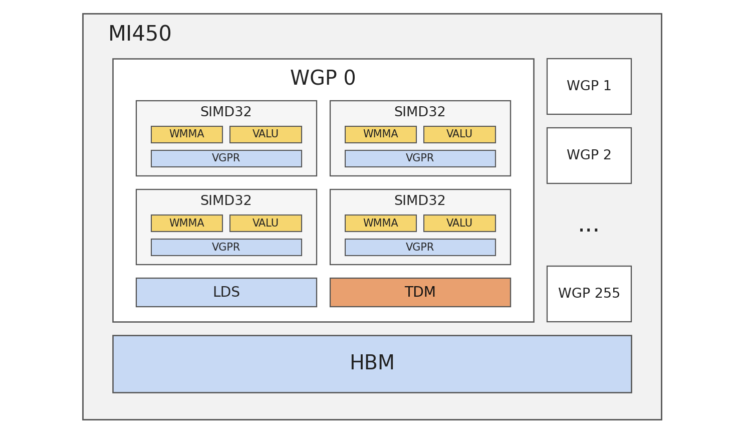
Kernel programmer view of the MI450 GPU hierarchy.

To write the MI450 kernel more efficiently, we will use Gluon in this blog. Gluon is a Triton-based DSL that keeps the tile-based SPMD programming model. Unlike Triton, tensors in Gluon must carry an explicit layout, which describes how each element is distributed across registers, lanes, waves, and workgroups. The layout also affects how the compiler generates instructions to move data among different memory hierarchies. This makes Gluon a lower-level programming language than Triton, and especially useful for kernel experts who want explicit control over generated instructions.

We assume the reader is familiar with the basics of Gluon semantics and its programming model. For Gluon kernel examples, please refer to the MI450 Gluon Examples.

Attention Decode Basics

With this hardware context in place, we can now turn to the workload: attention decode. We will start with a baseline attention decode kernel, then use it as the reference point for the optimizations in later sections. The attention operation can be expressed as follows: first, we perform a matrix multiplication of Q and K, then apply softmax to get P, and multiply P with V to get the final output O.

Attention formula.

In this blog, we use general 4D tensors to represent the attention inputs and outputs. For notation throughout this blog, B is the batch size, H_q is the number of Q heads, H_kv is the number of KV heads, T_q is the number of Q tokens, T_kv is the number of KV tokens, and D is the head dimension. The input QKV tensors are shown below.

Q: [B, H_q, T_q, D]
K: [B, H_kv, T_kv, D]
V: [B, H_kv, T_kv, D]

When H_q is equal to H_kv, we have standard multi-head attention (MHA), and when H_q is a multiple of H_kv, we have multi-query attention (MQA) or grouped-query attention (GQA). Modern LLMs often use MQA, such as GPT-OSS, so we will focus on MQA in this blog.

Attention in LLM inference includes two phases: prefill and decode. For prefill, T_q = T_kv, and the kernel can process many tokens in parallel. For decode, T_q = 1, but T_kv remains large and grows with the context length. Given each head is independent, standard MHA can waste a lot of compute resources for single-token decode.

However, in MQA decode, because multiple Q heads share one K and V head, the kernel can group those Q heads together. This can be reflected in the tensor shapes, as shown below, where the Q tensor is reshaped to group H_q / H_kv Q heads together for each KV head.

Q: [B, H_kv, H_q / H_kv, D]
K: [B, H_kv, T_kv, D]
V: [B, H_kv, T_kv, D]

Because tensors in each batch and each KV head are independent, we can process them in parallel. The kernel can be launched with a grid of (B, H_kv, 1), and each program processes a portion of the attention computation:

Q: [H_q / H_kv, D]
K: [T_kv, D]
V: [T_kv, D]

Following the Flash Attention algorithm, the kernel can compute one tile of K and V with shape (BLOCK_N, D) and one Q tile with shape (BLOCK_M, D) at a time, then slides through the T_kv dimension. The figure below shows an example workload with 2 batches and 2 KV heads. Each workgroup owns one (B, H_kv) pair, so there are 4 workgroups in total. Within each workgroup, multiple Q heads are processed together and shown as multiple rows. Here, we assume BLOCK_M = H_q / H_kv.

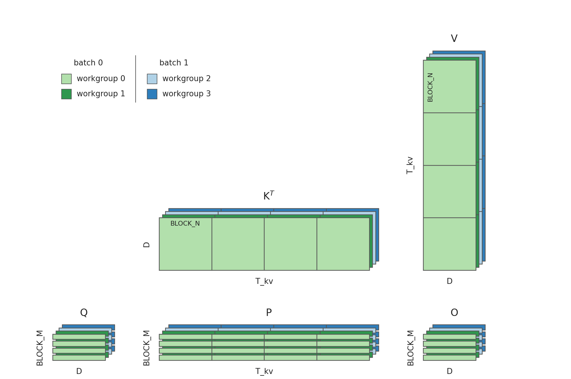
Attention decode workload mapping across batches and KV heads.

Decode Kernel Optimizations

So far, we have introduced a baseline implementation of an MQA decode kernel on MI450. This section will further discuss a series of optimizations that push the kernel toward peak performance on MI450. We will cover 4 major optimizations: tensor layout, data loading, pipelining, and parallelization with Split-k.

Optimize Tensor Layout

Gluon gives kernel authors explicit control over tensor layouts, which matters a lot for performance. A kernel can contain many different tensors, and deciding the right layout for each of them is non-trivial. In practice, the most important layout to decide first is the layout for the WMMA operands. In an attention kernel, there are two WMMA operations: QK and PV. We can start our layout optimization there.

In Gluon, AMDWMMALayout describes the WMMA output layout, and DotOperandLayout describes the WMMA operand layout. A given AMDWMMALayout determines the final WMMA instruction the compiler generates. For example, an AMDWMMALayout with instruction shape [16, 16, 128] for wmma_scaled generates v_wmma_scale_f32_16x16x128_f8f6f4 under the hood. This instruction consumes one FP8 operand of shape (16, 128), another FP8 operand of shape (128, 16), reduces over the K dimension of size 128, and produces a FP32 output tile of shape (16, 16) in one wave, where each element is assigned to a specific lane and register in this wave. The following figure shows how elements in the 2 WMMA operands and output tensor are assigned to lanes.

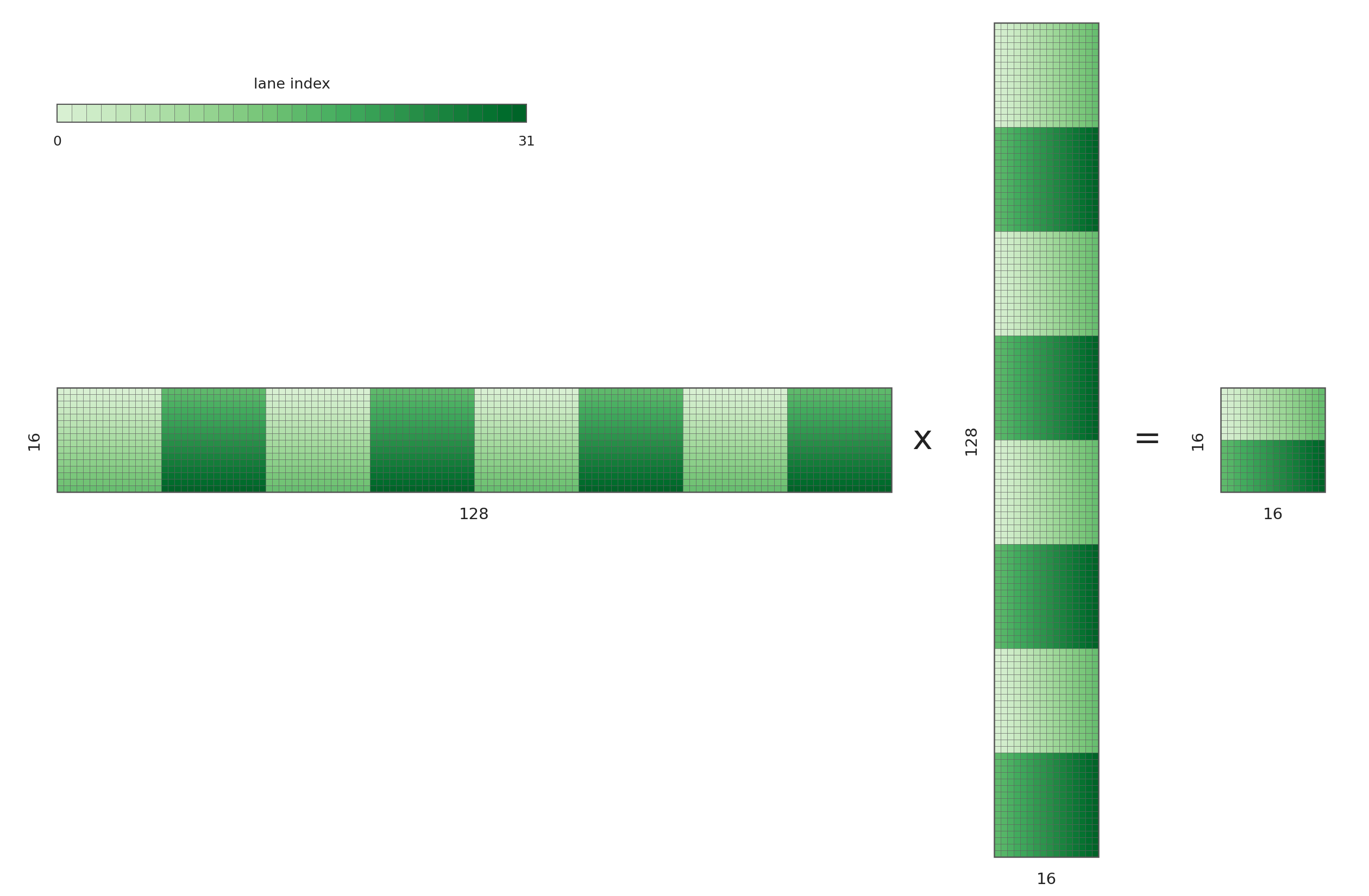
Lane assignment for the WMMA operands and output tile.

Next, we need to consider how waves are distributed. The kernel can use any power-of-two number of waves and distribute them across 2 dimensions of the WMMA output tile. Since online softmax reduces along T_kv dimension, we prefer to distribute waves along grouped Q dimension to avoid cross-wave communication during the reduction. In MQA decode, the Q tile has shape (H_q / H_kv, D), and H_q / H_kv is usually small, so we also need to avoid using too many waves there. For example, if H_q / H_kv = 32, the kernel chooses 2 waves, as shown below. In this figure, 2 waves have their own first WMMA operand, and share the second operand.

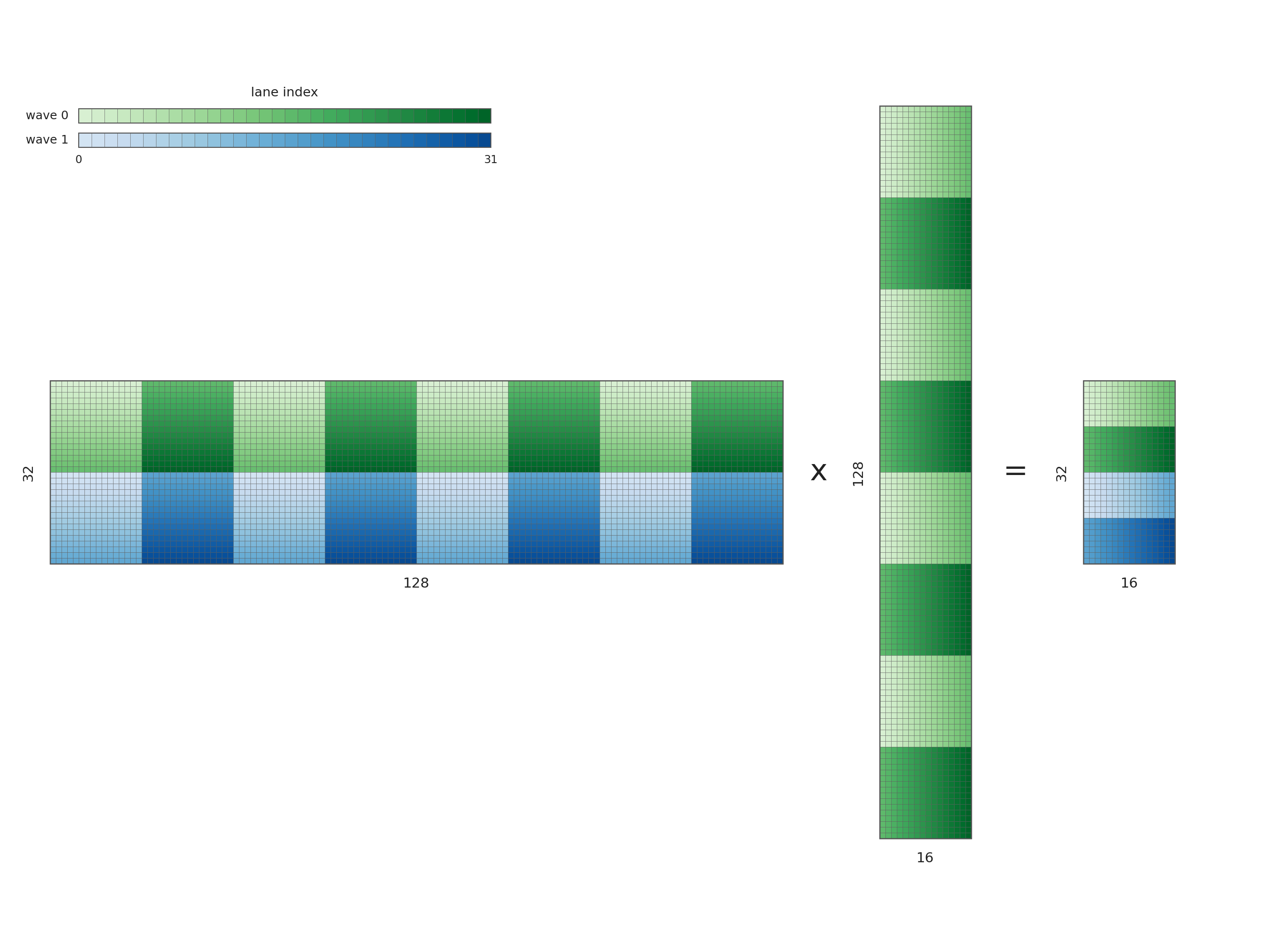
Two-wave WMMA layout with waves distributed across rows.

Another important factor to keep in mind is layout conversion. When two tensors in Gluon use different layouts, the kernel must use an explicit layout conversion operation to match them. Depending on the source and destination layouts, this conversion can happen in registers or through LDS. In attention, the output of the QK WMMA becomes the input of the PV WMMA after softmax. If the QK output layout is not compatible with the PV input layout, the hot loop pays an extra conversion cost. One useful technique is to “transpose” the WMMA output layout. This can be done by simply setting transpose=True in AMDWMMALayout, and the compiler will generate corresponding instruction to produce the transposed output. Note that this transpose operation does not incur extra instructions. For more details, please refer to this talk.

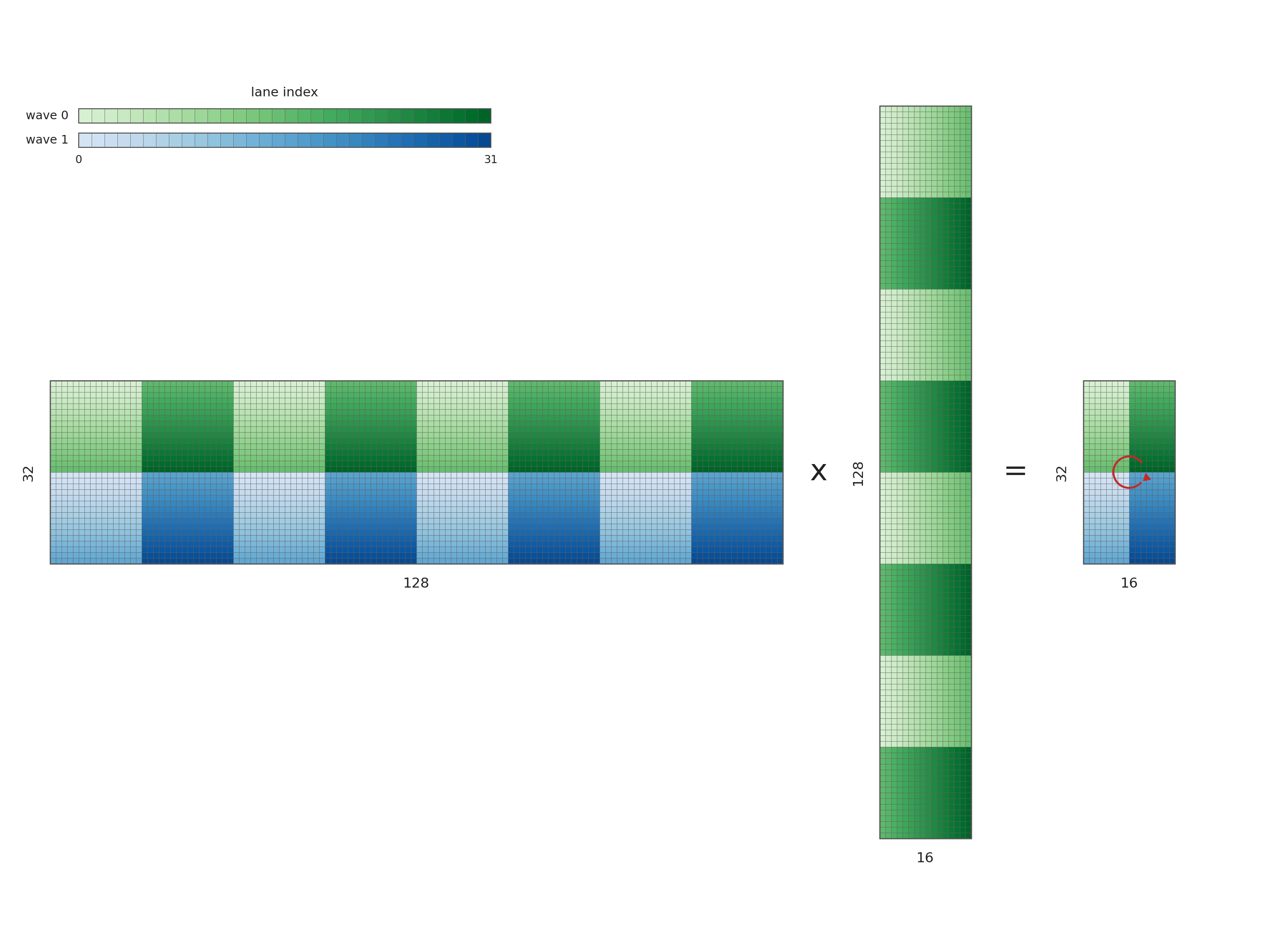
Transposed WMMA output layout for matching the PV input layout.

Another detail worth mentioning is the concept of “K Width”. In DotOperandLayout, K Width describes how many contiguous elements along the K dimension for WMMA should be assigned to one lane. A standard 16x16x128 WMMA instruction assumes K Width 16, but the transposed output for QK can have K Width 8. Therefore, we also need to explicitly set the PV input layout with K Width of 8 to match the QK output.

Optimize Data Loading

The hot loop of the decode kernel is dominated by loading K and V tiles from global memory to LDS. TDM helps accelerate this data path, but using TDM naively is not enough.

To understand the performance impact of TDM, we first need to understand the cache hierarchy on MI450. MI450 has a per-WGP cache at the same level as the LDS. But different from LDS, this cache is not directly visible to the programmer. TDM can either move data directly into the programmer-managed LDS or route the data through the cache path before it reaches the destination. Considering the limited size of the cache, memory-bound workloads are better off bypassing the cache and moving data directly into LDS.

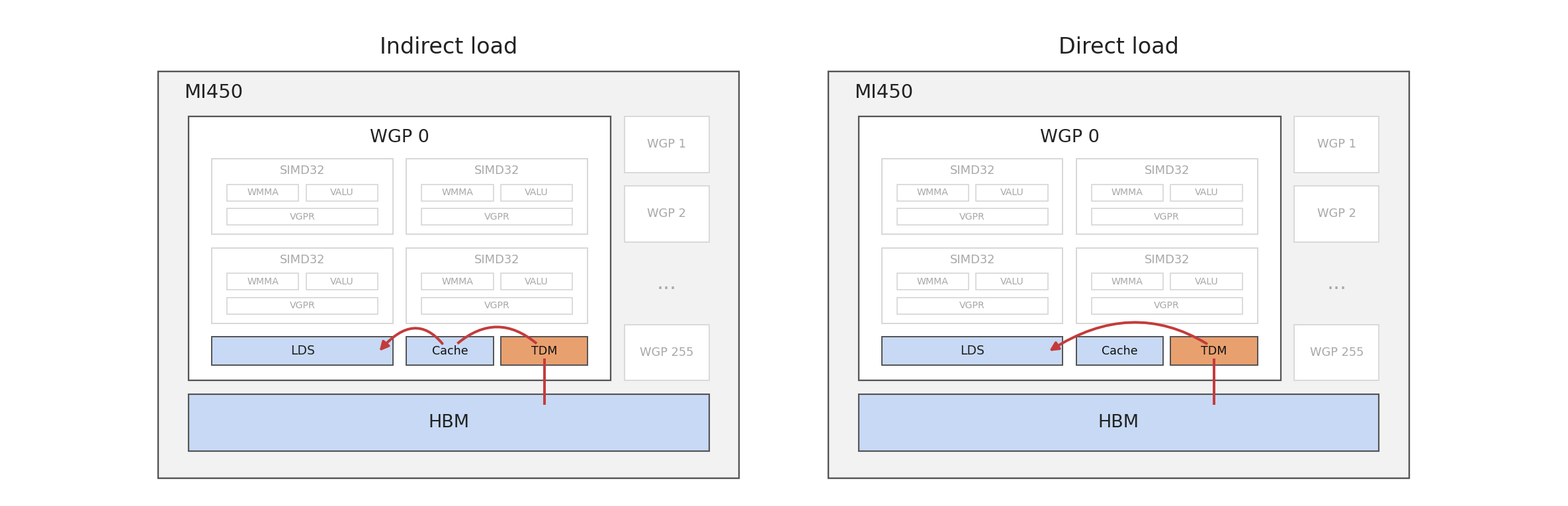
Indirect and direct TDM load paths on MI450.

Whether a TDM transfer uses the direct path depends on the shape of the TDM request. The innermost dimension needs to be at least 128 bytes to use the direct path, and 256 bytes is recommended to keep more in-flight memory traffic. Recall that K and V tiles have shape (BLOCK_N, D), so the innermost dimension is the head dimension D. Assuming an FP8 data type, this means the head dimension needs to be 256 for the optimal performance. In practice, head dimension is determined by the model architecture and cannot be changed by the kernel. However the kernel can reshape the K and V tensors to increase the innermost dimension before loading, then reshape them back while loading from LDS to registers. The following figure shows an example data flow of K and V for head dimension of 128.

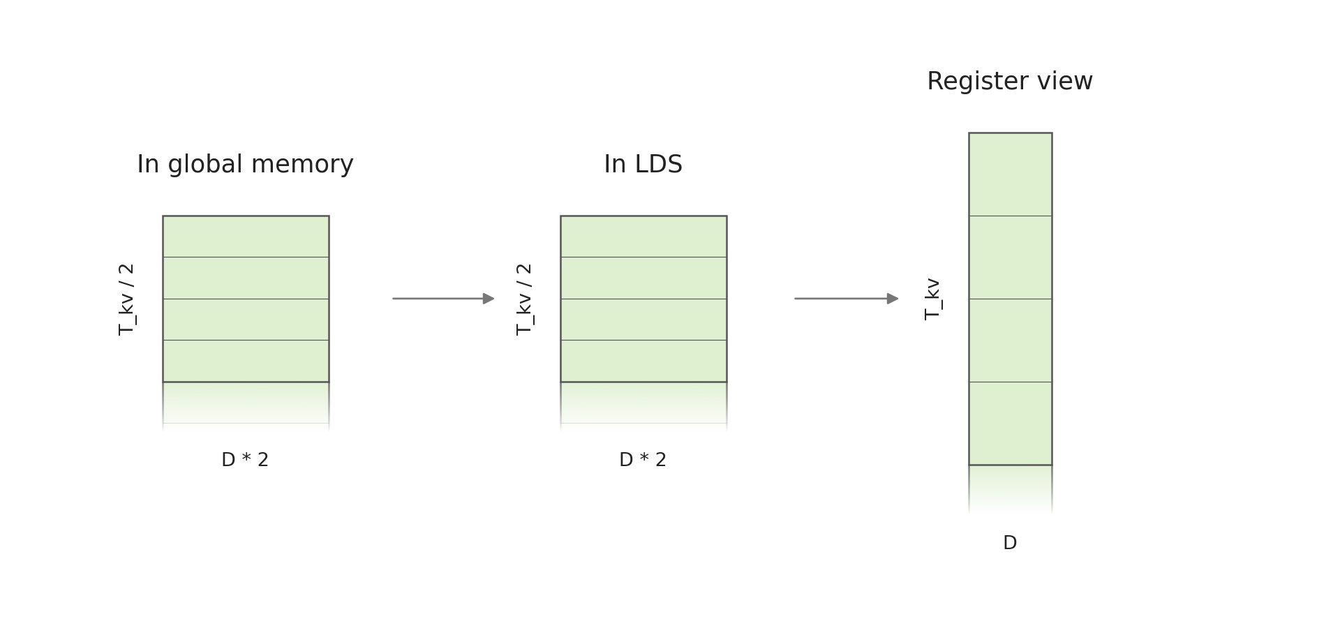
KV reshape used to create a wider TDM innermost dimension.

Pipeline for Latency Hiding

So far, we have optimized the tensor layout and data path. However, the hot loop can still stall on memory access latency. The next step is to pipeline the loop so that memory movement for one tile overlaps with computation for another tile.

To understand the pipeline, we can zoom into the attention formula shown earlier and write it in the tiled form used by the Flash Attention algorithm. The formula below shows one iteration i of the loop that processes one KV tile. Here we only focus on operations on 2D tiles, and omit operations on reduced 1D intermediate values. We use short operation names on the right side to denote each operation, making the pipeline easier to discuss later.

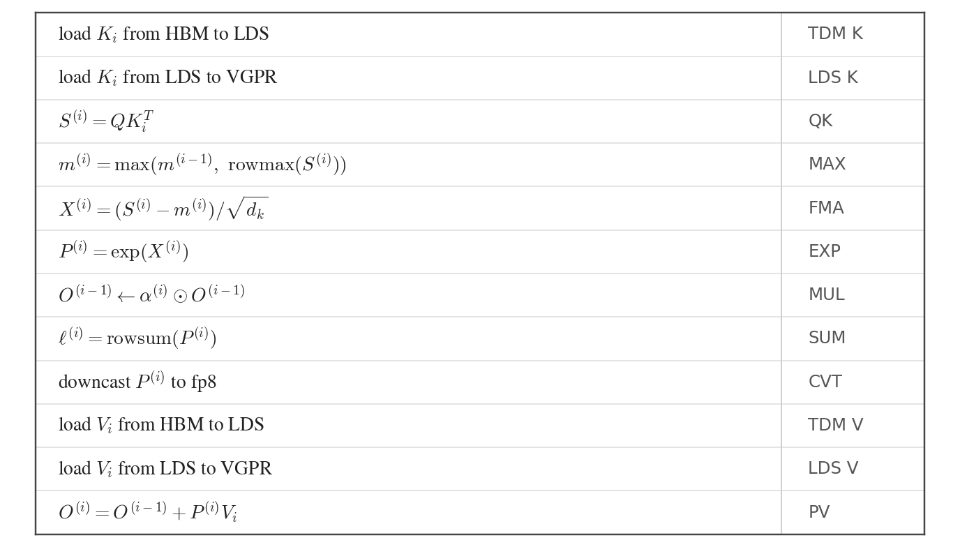
This figure shows one iteration i of the tiled attention loop, including only 2D operations. O, m, and l are loop-carried intermediate values for online softmax. The right side shows the short operation names used in the pipeline discussion.

Each line in the figure can be expressed as one Gluon operation, which will be expanded to a sequence of instructions. The following table shows the expanded instruction groups for FP8 decode attention with BLOCK_M = 32, BLOCK_N = 128, D = 128, and two waves. The Cycles column gives a simplified per-instruction cost estimate based on hardware specifications. Memory instructions are left blank because their latency is modeled separately.

Operation	Instruction	Count	Cycles
TDM K	tensor_load_to_lds	1
LDS K	ds_load_b128	32
QK	v_wmma_scale_f32_16x16x128_f8f6f4	8	8
MAX	v_maximum3_f32	32	1
FMA	v_pk_fma_f32	32	1
EXP	v_exp_f32	64	2
SUM	v_pk_add_f32	32	1
MUL	v_pk_mul_f32	32	1
CVT	v_cvt_scalef32_pk8_fp8_f32	8	4
TDM V	tensor_load_to_lds	1
LDS V	ds_load_tr8_b64	64
PV	v_wmma_scale_f32_16x16x128_f8f6f4	8	8

This table gives us the basic scheduling units. The goal of pipelining is to move independent units from different loop iterations into the same time window.

Our first attempt is to separate memory movement from computation. In the simple two-stage pipeline below, one stage issues TDM loads for future iterations, while the other stage consumes data that has already arrived in LDS. The notation [i] means the operation belongs to loop iteration i. This schedule needs double buffering. While one LDS buffer is being consumed by LDS loads and WMMA, the other buffer can be filled by TDM for a later iteration. On the next loop step, the two buffers swap roles.

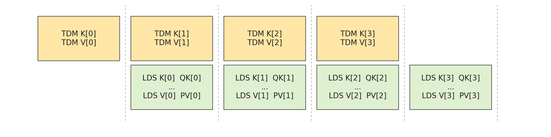
Two-stage pipeline schedule.

The two-stage pipeline can overlap TDM loads with computation. This works well when the loop is clearly memory-bound, but it treats the entire compute side as one monolithic block. As a result, LDS loads, WMMA for QK, WMMA for PV, a series of vector instructions for softmax are effectively serialized inside the compute stage. This unnecessarily inflates the compute block. In the worst case, the kernel can shift from being limited by TDM latency to being limited by serialized compute.

To avoid this, we split the compute block according to the actual data dependencies. These operations do not all depend on the same values or use the same hardware resources, so WMMA instructions, LDS movement, and softmax vector work can often be interleaved once their operands are ready. In the dependency graph below, each node is one scheduling unit. An edge means the destination cannot start until the source has produced its value.

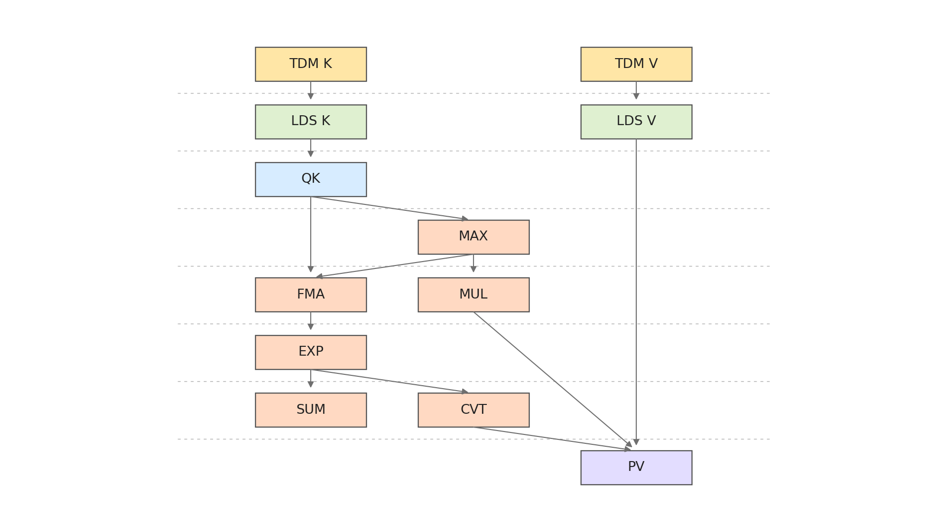
Data dependencies among the scheduling units in one loop iteration.

We can observe that the QK for iteration i + 1 does not need the softmax result from iteration i, so the next KV tile can be prefetched and its QK computation can start earlier. Moreover, QK and PV use WMMA instructions, while the online softmax only uses VALU instructions, so these operations can be interleaved instead of serialized.

These observations motivate the four-stage pipeline. Instead of putting all non-TDM work into one compute stage, the four-stage pipeline interleaves memory and compute units from neighboring iterations. A stage may contain QK from iteration i + 1, softmax work from iteration i, an LDS load for iteration i, and a TDM request for a future iteration. We group the softmax work into two stages with roughly equal amount of work, to help hardware better interleave WMMA and VALU. Here, QK WMMA can interleave with VEC0 and PV WMMA can interleave with VEC1. In addition, EXP uses the transcendental unit and can be further interleaved with other VALU instructions.

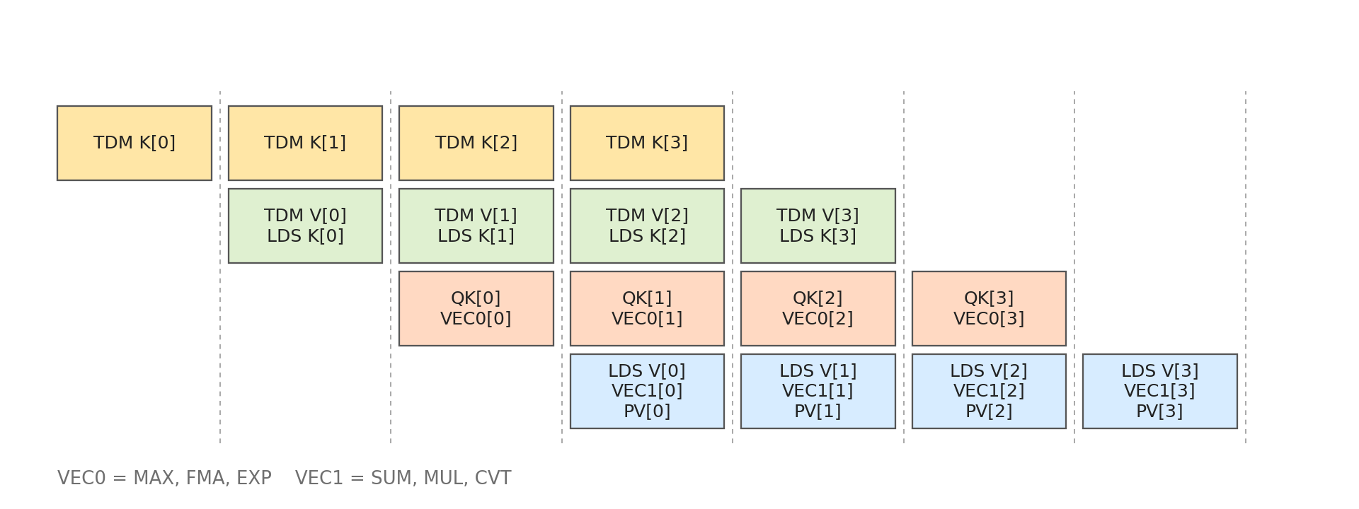
Four-stage pipeline schedule with double buffering.

This four-stage schedule exposes more overlap than the two-stage schedule, but it still leaves one question: how far ahead should the TDM requests be issued? With double buffering, the kernel has 2 LDS slots. One slot is being consumed by LDS loads and compute, while the other slot is being filled by TDM. This gives each TDM request roughly one iteration of compute time before the data is needed.

We can estimate whether that is enough with a simple cycle model. Assume TDM load takes about 1000 cycles and all LDS load latency can be hidden by scheduling. Using this model and the previous table, we can get the following estimate for one decode iteration shown in the table below. Here we use 2 interleave rules: 1) one WMMA takes 8 cycles, and can hide 2 cycles of VALU; 2) one EXP takes 2 cycles, and can hide 1 cycle of non-EXP VALU. Also note this 1000 cycles is an empirical number to help us reason about the pipeline. The actual TDM latency depends on many factors, like the tensor tile shape and access pattern.

Group	Total Cycles
QK	64
PV	64
VEC0 = MAX + FMA + EXP	192
VEC1 = SUM + MUL + CVT	96
QK + VEC0, interleaved	176
PV + VEC1, interleaved	144
Total, interleaved	320

In a double-buffered schedule, a TDM request has roughly 320 cycles of effective compute work to overlap with before the loaded tile is consumed. This is much smaller than the 1000-cycle TDM latency in this model, leaving about 680 cycles of exposed wait for each load.

This motivates a longer lookahead distance. Triple buffering adds one more LDS slot, so the kernel can request a future tile earlier instead of waiting for the next buffer swap. Conceptually, one buffer is being consumed, one buffer is ready or close to ready, and one buffer is being filled by TDM. In the same model, looking ahead by two iterations gives about 640 cycles of effective compute work to overlap. It still does not cover the full memory latency, but it reduces the exposed wait from about 680 cycles to about 360 cycles and gives the hardware more outstanding memory work.

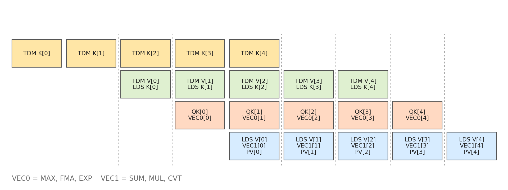
Four-stage pipeline with triple buffering.

Parallelize with Split-k

The pipeline optimizes latency hiding inside one workgroup, but one GPU has many workgroups, and we also need to make sure we can saturate the full GPU memory bandwidth across all workgroups. In the baseline MQA/GQA decode mapping, each workgroup owns one (B, H_kv) pair and walks through that pair’s KV sequence serially. The total number of workgroups is only B * H_kv. On MI450, there are 256 workgroup processors, so small batch sizes or small numbers of KV heads may launch too few workgroups to fully utilize the available memory bandwidth.

Split-k addresses this under-utilization problem by partitioning the KV sequence across multiple workgroups. Instead of assigning the whole KV sequence for one (B, H_kv) pair to a single workgroup, Split-k divides it into S partitions and lets S workgroups process those partitions in parallel. The number of workgroups increases from B * H_kv to B * H_kv * S, improving GPU saturation while also reducing the number of KV blocks handled by each workgroup. The partial results from the partitions are then merged to produce the final attention output. The following figure shows an example with 2 batches, 2 KV heads, and 2 partitions: the total number of workgroups doubles, and each workgroup processes half of the KV sequence.

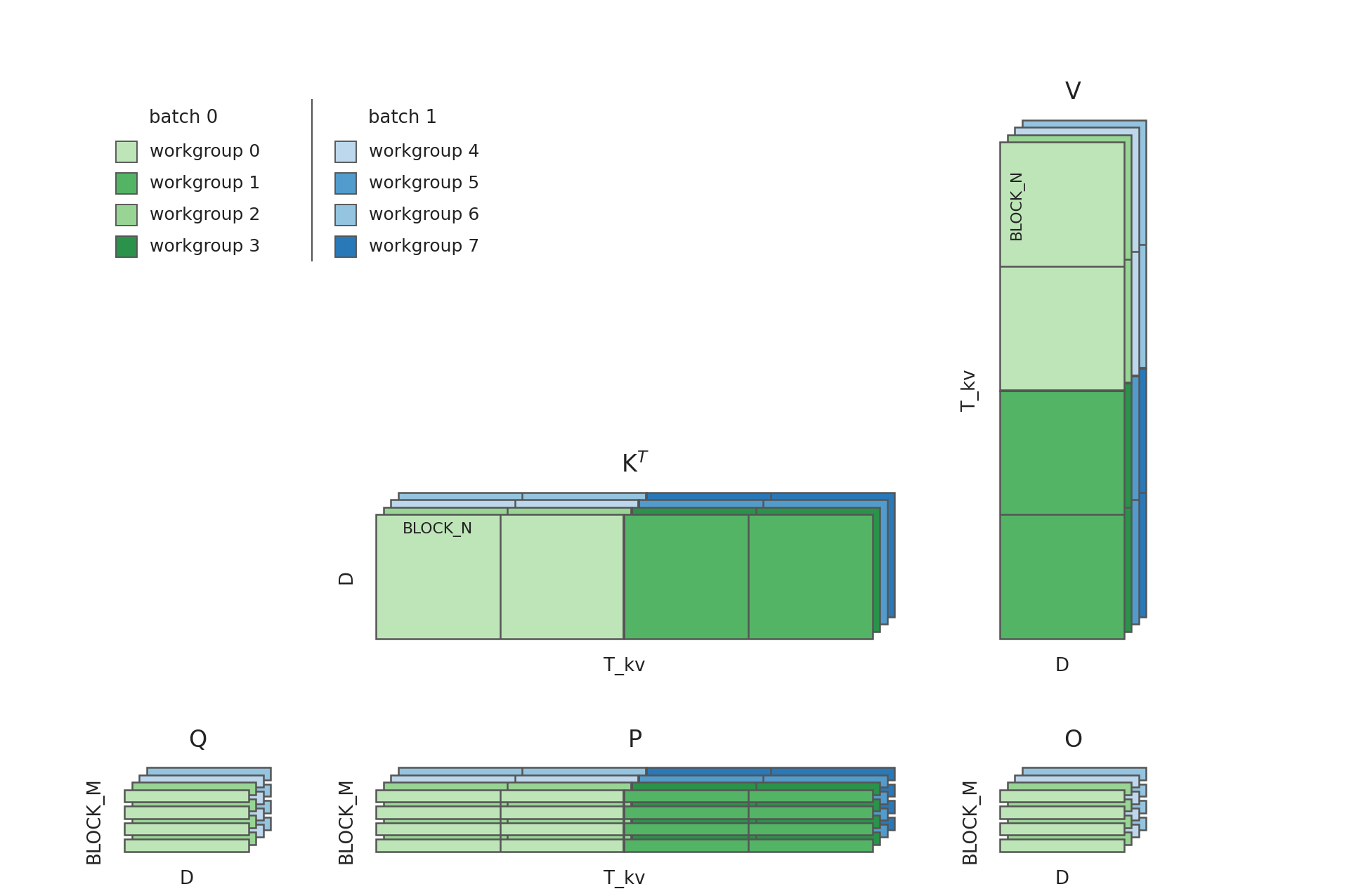
Split-k workload mapping across K/V sequence partitions.

One challenge with Split-k is that all workgroups also need to synchronize and merge their partial results. Typically, there is a separate reduction kernel to merge the partial results. This two-kernel approach uses global memory to store the intermediate results and also sets a natural synchronization point. MI450 introduces the new workgroup cluster feature, which allows a cluster of workgroups to synchronize. We can use this feature to implement Split-k in a single kernel by fusing the reduction compute.

In Gluon, the concept of a workgroup cluster is expressed via multi-CTA programming. “CTA” is the Triton term for a workgroup, and “CGA” is the term for a cluster. The following table shows the mapping between Triton and MI450 concepts:

Triton Concept	MI450 Concept
Warp	Wavefront
CTA	Workgroup
CGA	Workgroup Cluster

Gluon kernels distribute CTAs just like warps; both are part of the layout system. One detail to note is that when discussing block size in Triton, it usually means the block size of one workgroup. With a multi-CTA layout, the block size is the size of the whole cluster.

Layouts in Gluon, such as AMDWMMALayout, allow specifying the cga_layout field for the multi-CTA kernel. In the Split-k case, since each workgroup processes a partition independently until the final reduction, we can perform the partial attention in 3D format. Effectively, each program processes the attention computation shown below. All partitions here share the same Q.

Q: [1, H_q / H_kv, D]
K: [S, T_kv / S, D]
V: [S, T_kv / S, D]

To see how this maps to the layout system, it is useful to look at a single WMMA operation under a multi-CTA layout. In the figure below, we add one extra dimension to the WMMA layout for workgroups. The first operand is shared across 2 partitions. The second operand and output are different. Within each workgroup, the two waves are still distributed as before.

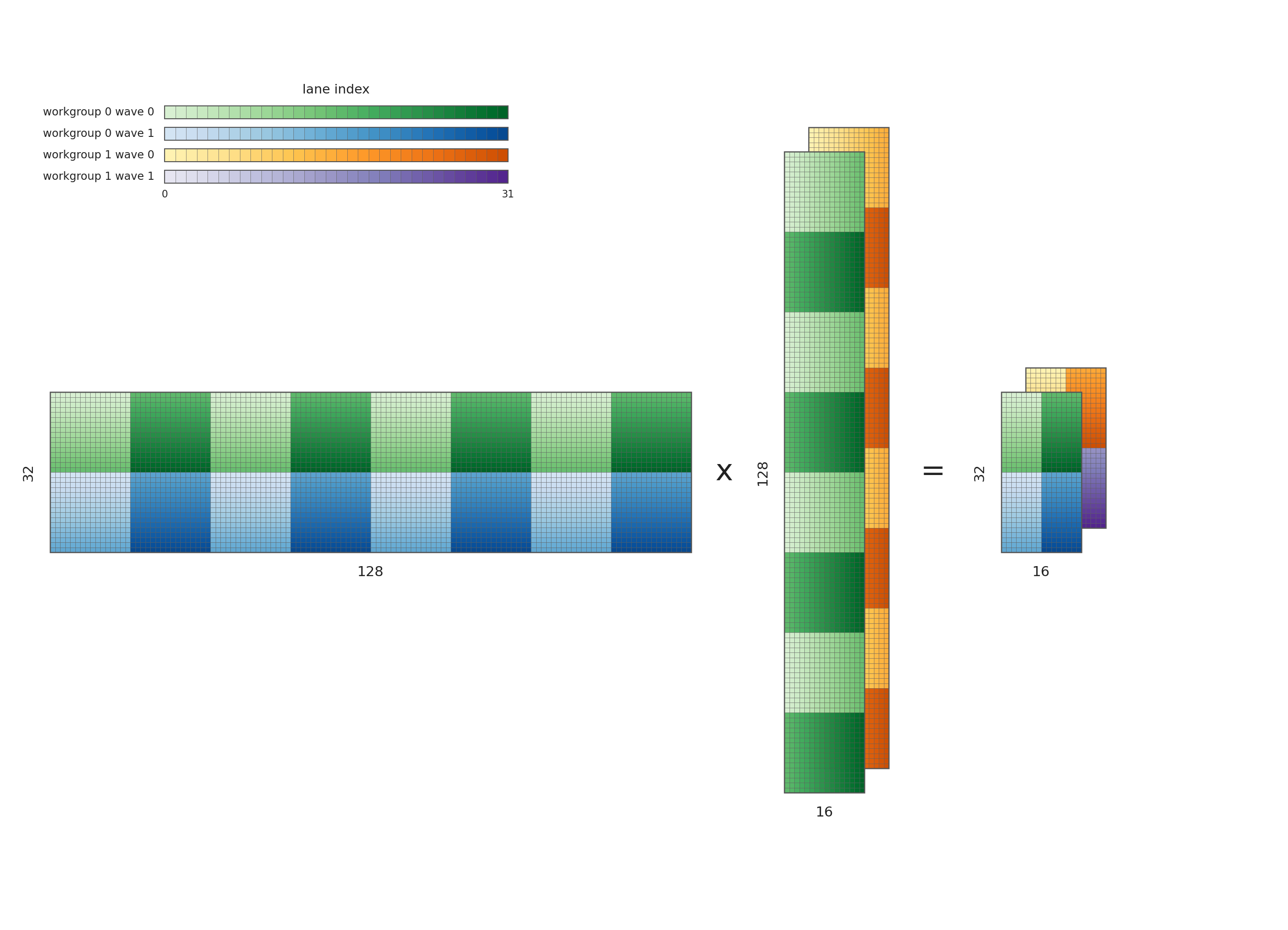
Multi-CTA WMMA layout for split-k attention.

After the partial attention, we need to merge the results from all workgroups. The kernel will first write the partial results to global memory, synchronize all workgroups in the cluster, and finally read back the partial results. It is also worth mentioning that MI450 provides the L2 cache which is shared across workgroups in a cluster. So the partial results do not need to be passed through global memory. This helps to cut the overhead of the reduction.

As the reduction is fused into the same kernel, we will use the same launch grid for the reduction, but with a different layout. Workgroups are now distributed along the head dimension and loop through each partition to compute the final result.

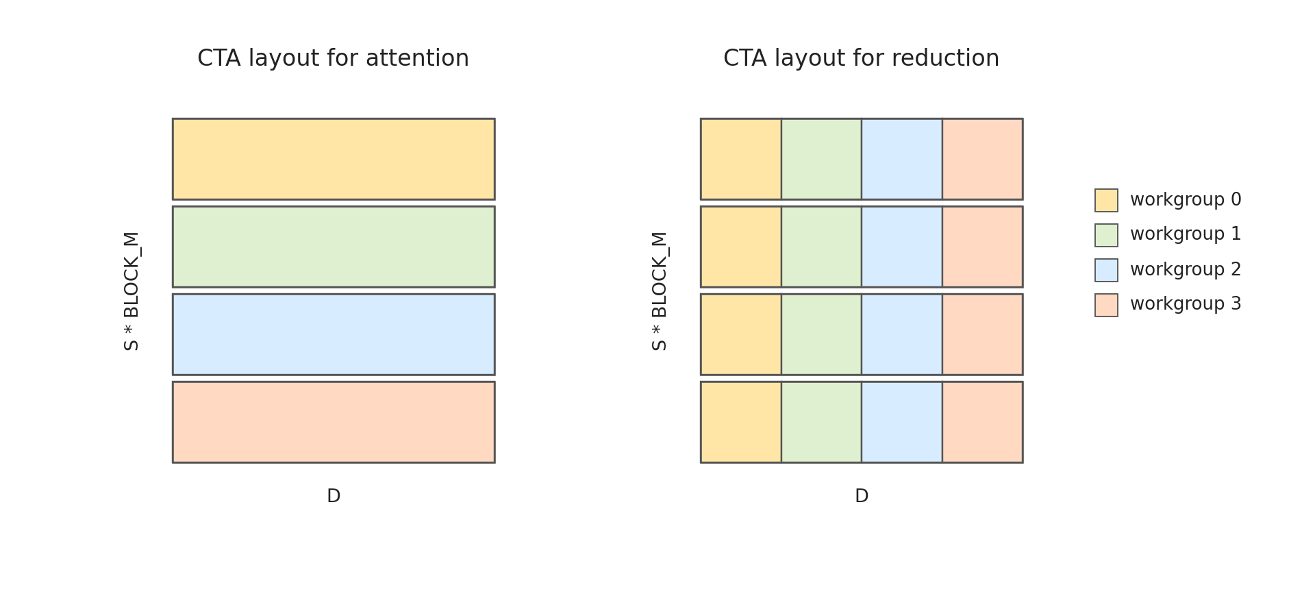
CTA layouts for split-k attention and reduction.

Performance Evaluation

So far, we have covered the main optimization steps for MQA decode on MI450, including:

1. Optimize tensor layout: Choose optimal Gluon layouts to help the compiler generate better instructions;

2. Optimize data loading: Optimize K/V TDM requests to speed up memory access;

3. Pipeline for latency hiding: Overlap memory access, matrix multiplication, and softmax to reduce exposed memory latency;

4. Parallelize with Split-k: Split the KV sequence across multiple workgroups to fully utilize the GPU memory bandwidth.

Apart from all the optimizations discussed above, the kernel also uses a few other techniques to improve performance, including better code generation and underlying instruction-level optimizations in LLVM.

We implemented the above optimizations in a Gluon kernel. The kernel source code is fully open source in the MI450 Gluon MXFP Attention Example. Our evaluation of this kernel covers the following target settings:

• Batch: 64

• Number of Q heads: 64

• Number of KV heads: 1 or 2

• KV sequence length: 4096-65536

• QKV data type: FP8 with a global scale

We use the effective bandwidth of the kernel as the target metric, defined as the total number of bytes read and written to global memory divided by the total kernel execution time. For a system-level memory-bandwidth reference, we also measured the peak read-only bandwidth on the same MI450 system using the BabelStream. The following figure shows the performance of the kernel for the target settings:

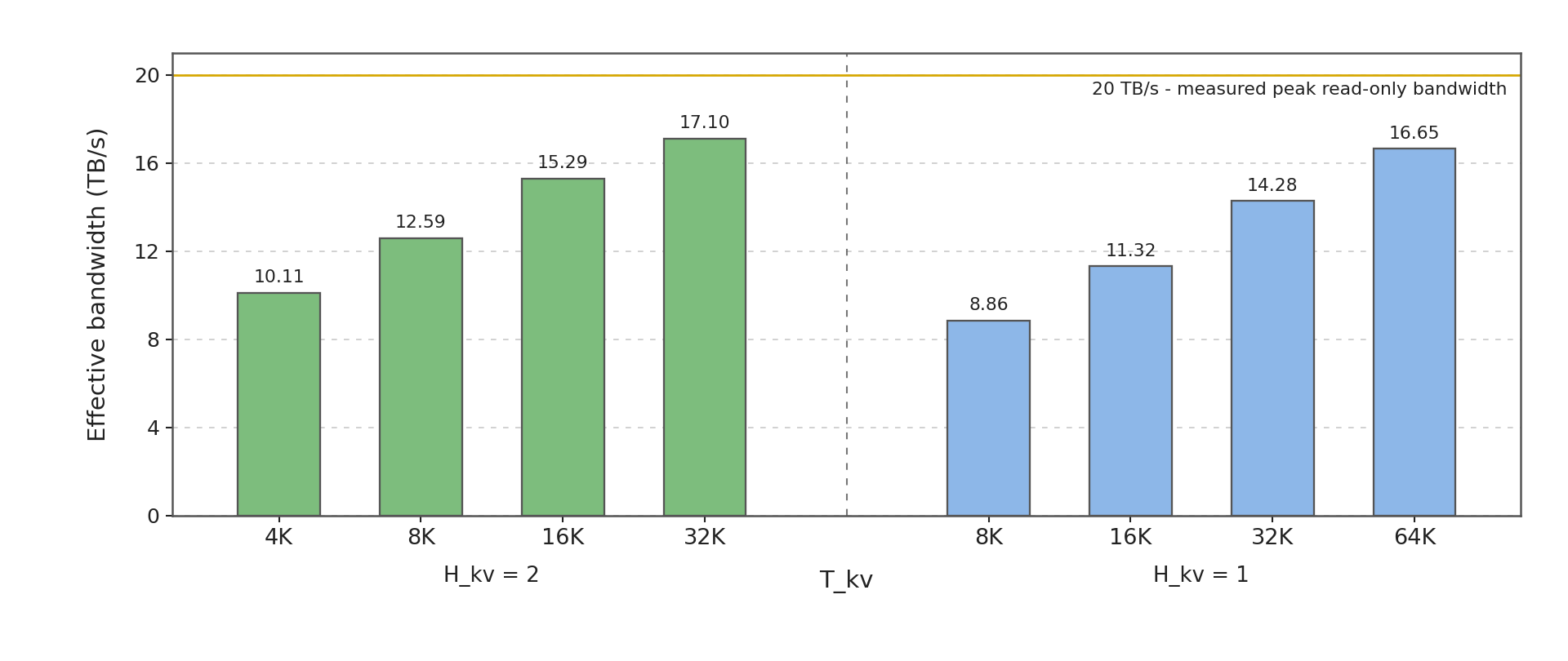
Effective bandwidth of the optimized attention decode kernel on MI450.

The reported peak bandwidth on our evaluation system is 20TB/s. In the GQA case with H_kv = 2, effective bandwidth reaches 17.10 TB/s, 85% of the peak bandwidth. In the MQA case with H_kv = 1, the kernel reaches 16.65 TB/s, 83% of the peak bandwidth. The throughput of the kernel increases with sequence length. At shorter sequence lengths, fixed costs such as prologue and reduction overhead take a larger fraction of the total runtime.

The above results were collected with ROCm 7.14.0 and PyTorch 2.11.0, using Triton commit ecfc626 with the latest mxfp_fa_gfx1250.py script. To reproduce the results, please run the following command:

# H_kv = 2
python3 third_party/amd/python/examples/gluon/mxfp_fa_gfx1250.py --q_type e4m3 --kv_type e4m3 --batch 64 --seqlen_q 1 --seqlen_k 4096 --num_q_heads 64 --num_k_heads 2 --head_sz 128 --pipelined --scale_type global --profile
python3 third_party/amd/python/examples/gluon/mxfp_fa_gfx1250.py --q_type e4m3 --kv_type e4m3 --batch 64 --seqlen_q 1 --seqlen_k 8192 --num_q_heads 64 --num_k_heads 2 --head_sz 128 --pipelined --scale_type global --profile
python3 third_party/amd/python/examples/gluon/mxfp_fa_gfx1250.py --q_type e4m3 --kv_type e4m3 --batch 64 --seqlen_q 1 --seqlen_k 16384 --num_q_heads 64 --num_k_heads 2 --head_sz 128 --pipelined --scale_type global --profile
python3 third_party/amd/python/examples/gluon/mxfp_fa_gfx1250.py --q_type e4m3 --kv_type e4m3 --batch 64 --seqlen_q 1 --seqlen_k 32768 --num_q_heads 64 --num_k_heads 2 --head_sz 128 --pipelined --scale_type global --profile

# H_kv = 1
python3 third_party/amd/python/examples/gluon/mxfp_fa_gfx1250.py --q_type e4m3 --kv_type e4m3 --batch 64 --seqlen_q 1 --seqlen_k 8192 --num_q_heads 64 --num_k_heads 1 --head_sz 128 --pipelined --scale_type global --profile
python3 third_party/amd/python/examples/gluon/mxfp_fa_gfx1250.py --q_type e4m3 --kv_type e4m3 --batch 64 --seqlen_q 1 --seqlen_k 16384 --num_q_heads 64 --num_k_heads 1 --head_sz 128 --pipelined --scale_type global --profile
python3 third_party/amd/python/examples/gluon/mxfp_fa_gfx1250.py --q_type e4m3 --kv_type e4m3 --batch 64 --seqlen_q 1 --seqlen_k 32768 --num_q_heads 64 --num_k_heads 1 --head_sz 128 --pipelined --scale_type global --profile
python3 third_party/amd/python/examples/gluon/mxfp_fa_gfx1250.py --q_type e4m3 --kv_type e4m3 --batch 64 --seqlen_q 1 --seqlen_k 65536 --num_q_heads 64 --num_k_heads 1 --head_sz 128 --pipelined --scale_type global --profile

Summary

In this blog, we used attention decode as a case study to walk through the main optimization steps for MI450. We started from a baseline attention loop, then optimized the WMMA layouts, data loading, and software pipelining. We also discussed how to use split-k with workgroup clusters to increase parallelism for long-context decode. The optimized attention decode kernel can reach 85% of the peak memory bandwidth on MI450. This is an early result, and we expect to further improve the kernel performance with more optimizations in the future, such as memory prefetching, better instruction-level scheduling and improved reduction for split-k.

We also demonstrated that MI450 provides several hardware features that are especially useful for decode workloads: TDM for asynchronous global-to-LDS movement, larger register and LDS resources, and workgroup clusters for cooperation across workgroups. Gluon exposes all of these features and allows kernel authors to perform low-level optimizations while maintaining a tile-based SPMD programming model consistent with Triton. This opens up many optimization opportunities for kernel experts to achieve peak performance on MI450.

Moving forward, we plan to continue to apply these optimization techniques to other attention decode kernels, covering different data types, paged KV cache, and also different attention variants like MLA/DSA kernels in the DeepSeek family. These kernels will be further pushed to production-ready quality and integrated into LLM inference frameworks.

Disclaimers

The information presented in this document is for informational purposes only and may contain technical inaccuracies, omissions, and typographical errors. The information contained herein is subject to change and may be rendered inaccurate for many reasons, including but not limited to product and roadmap changes, component and motherboard version changes, new model and/or product releases, product differences between differing manufacturers, software changes, BIOS flashes, firmware upgrades, or the like. Any computer system has risks of security vulnerabilities that cannot be completely prevented or mitigated. AMD assumes no obligation to update or otherwise correct or revise this information. However, AMD reserves the right to revise this information and to make changes from time to time to the content hereof without obligation of AMD to notify any person of such revisions or changes. THIS INFORMATION IS PROVIDED ‘AS IS.” AMD MAKES NO REPRESENTATIONS OR WARRANTIES WITH RESPECT TO THE CONTENTS HEREOF AND ASSUMES NO RESPONSIBILITY FOR ANY INACCURACIES, ERRORS, OR OMISSIONS THAT MAY APPEAR IN THIS INFORMATION. AMD SPECIFICALLY DISCLAIMS ANY IMPLIED WARRANTIES OF NON-INFRINGEMENT, MERCHANTABILITY, OR FITNESS FOR ANY PARTICULAR PURPOSE. IN NO EVENT WILL AMD BE LIABLE TO ANY PERSON FOR ANY RELIANCE, DIRECT, INDIRECT, SPECIAL, OR OTHER CONSEQUENTIAL DAMAGES ARISING FROM THE USE OF ANY INFORMATION CONTAINED HEREIN, EVEN IF AMD IS EXPRESSLY ADVISED OF THE POSSIBILITY OF SUCH DAMAGES. AMD, the AMD Arrow logo, and combinations thereof are trademarks of Advanced Micro Devices, Inc. Other product names used in this publication are for identification purposes only and may be trademarks of their respective companies. © 2026 Advanced Micro Devices, Inc. All rights reserved

Cautionary Statement

This blog may contain forward-looking statements concerning Advanced Micro Devices, Inc. (AMD), which are made pursuant to the Safe Harbor provisions of the Private Securities Litigation Reform Act of 1995. Forward-looking statements are commonly identified by words such as “would,” “may,” “expects,” “believes,” “plans,” “intends,” “projects” and other terms with similar meaning. Investors are cautioned that any forward-looking statements in this blog are based on current beliefs, assumptions and expectations, speak only as of the date of this blog and involve risks and uncertainties that could cause actual results to differ materially from current expectations. Such statements are subject to certain known and unknown risks and uncertainties, many of which are difficult to predict and generally beyond AMD’s control, that could cause actual results and other future events to differ materially from those expressed in, or implied or projected by, the forward-looking information and statements. Investors are urged to review in detail the risks and uncertainties in AMD’s Securities and Exchange Commission filings, including but not limited to AMD’s most recent reports on Forms 10-K and 10-Q.

AMD does not assume, and hereby disclaims, any obligation to update forward-looking statements made in this blog, except as may be required by law.