Primus-Pipeline: A More Flexible and Scalable Pipeline Parallelism Implementation

February 23, 2026 by Cheng Yao, Lihuan Zhang, Wen Xie, Xiaoming Peng, Yuankai Chen, Anshu Raina, Chaojun Hou, Yao Fu, Liz Li, Zhenyu Gu.

5 min read. | 1207 total words.

Software tools & optimizations

AI/ML, LLM, Optimization

Developers, AI, Systems

This blog covers a flexible pipeline parallelism implementation in the Primus Megatron-LM backend, which supports a full stack of zero-bubble algorithms including zerobubble/zbv/v-half/v-min, as well as traditional 1f1b and 1f1b-interleaved schedules. We also provide a full stack of simulation and performance tools to analyze pipeline scheduling algorithms in both theory and practice.

Background

Pipeline parallelism (PP) is an efficient strategy for large language model pretraining. For models that must span multiple nodes, pipeline parallelism enables model sharding with primarily neighbor point‑to‑point activation transfers (instead of heavy global collectives), often improving the scalability and predictability of scale‑out communication.

1f1b and 1f1b-interleaved are two PP scheduling algorithms widely used in LLM training frameworks such as Megatron-LM and DeepSpeed. In recent years, several state-of-the-art pipeline parallelism methods have been proposed, such as the zero-bubble algorithm by Sea AI Lab and DualPipe/DualPipe-V by the DeepSeek team, but they are not integrated into open-source LLM training frameworks mainly because the scheduling logic is fixed and hard to modify.

For example, in the Megatron-LM 1f1b-interleaved implementation, the PP schedule is depicted by three main loops: warm-up, the 1f1b steady phase, and cool down. The warm-up phase executes only forward passes, the steady phase executes one forward and one backward in order, and finally the cool down phase executes the last mini-batches’ backward passes. Communication nodes are inserted inside the loop. In this case, if you want to add a new schedule such as zero-bubble or dual-pipe, you need to copy the three loops and modify their details, which can become long and complicated.

Primus-Pipeline

The key idea of Primus-Pipeline is to separate pipeline scheduling logic from training execution, making it convenient to verify and implement new pipeline schedule algorithms. Our main contributions can be summarized in the following three points.

• Provide a flexible abstraction for PP scheduling algorithms and fully support many state-of-the-art algorithms, including 1f1b-interleaved and zero-bubble based schedules.

• Implement Input Gradient/Weight Gradient separation ops for GEMM and Grouped GEMM by redefining Primus-Turbo ops.

• Provide simulation tools for each PP algorithm in both theory and practice, which clearly simulate and measure bubble rate and memory consumption under specific configs.

Schedule Design

Primus-Pipeline patches and substitutes the Megatron-LM’s megatron.core.pipeline_parallel.get_forward_backward_func function. The entry point of the schedule logic is at PrimusPipelineParallelLauncher

Here are the steps to define and run a PP algorithm in Primus-Pipeline.

1. Create a ScheduleTable with ScheduleNodes: For most PP algorithms, a schedule table containing schedule nodes can be defined given PP world size, virtual pipeline chunks per rank, and mini-batches.

   • Schedule Nodes: Each step of the execution can be abstracted as a schedule node including computation nodes such as FORWARD/BACKWARD/WGRAD(calculate the weights’ gradients) and communication nodes such as RECEIVE_FORWARD/SEND_FORWARD.

   • PP Algorithms: pp-algorithms

2. Bind the Schedule Nodes with their execution functions and arguments: Each node in the schedule table is bound to its handler functions and runtime arguments. For example, Primus binds Megatron-LM backend functions in this code. Megatron-LM backend binding

3. Launch the ScheduleRunner: After binding execution functions on the schedule table, it is launched by ScheduleRunner

Simulator and perf

To validate and compare the performance of different PP algorithms, we offer tools that can perform projections without hardware and also observe and profile PP schedules in real runs.

Simulator

Given a ScheduleTable, the simulator estimates bubble rate, memory footprint, and timing based on a provided configuration without requiring physical devices. This enables rapid comparison of different schedule designs and iterative development before running full-scale experiments.

Below is an example demonstrating how to validate different PP algorithms using the configuration defined in pp_simulation.yaml. We also did a lot of works on fine-grained projections with transformer layer performance metrics and various parallel strategies, please refer to the projection readme.

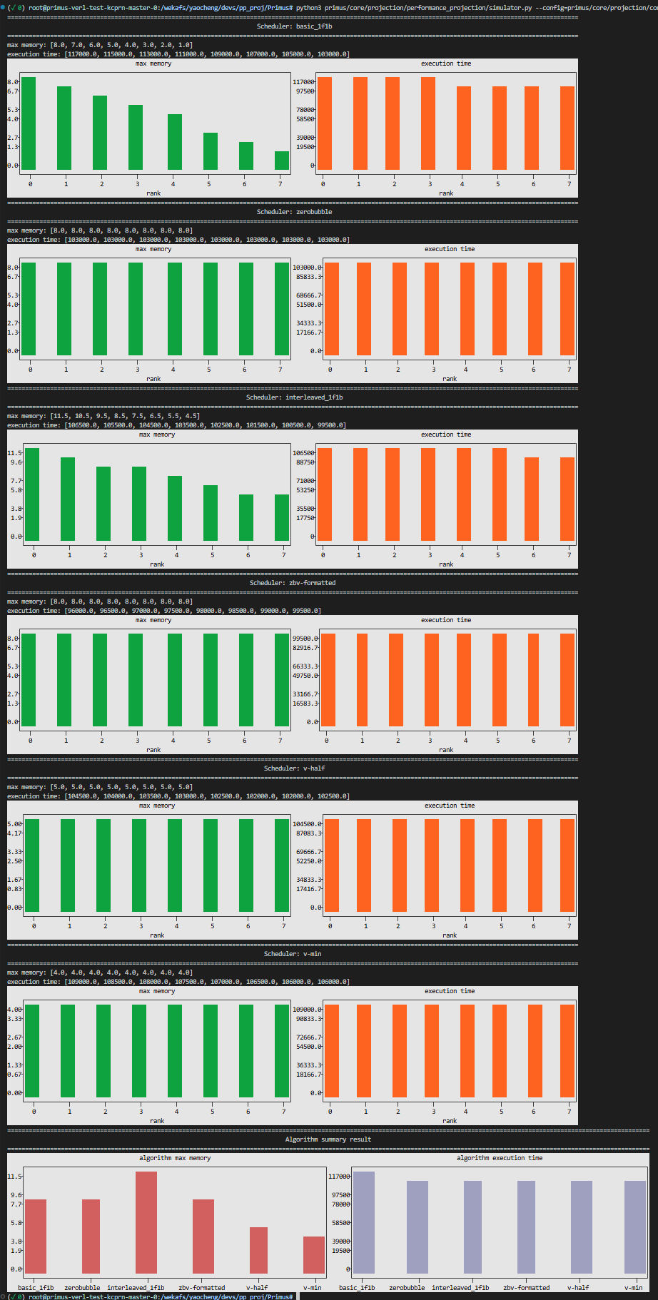
Execute the command below to run the simulation program. The tool will output performance metrics for different algorithms directly in the console. The data generated by the simulator can be visualized by visualization tools introduced in the next section.

python3 primus/core/projection/performance_projection/simulator.py --config=primus/core/projection/configs/pp_simulation.yaml

Below is the output of the simulator.py for the configuration with 8 pipeline stages and different algorithms.

Perf & Visualization tools

We provide tools to analyze and visualize pipeline parallelism schedules in two modes: using simulator output for offline analysis, or using data dumped from real training runs.

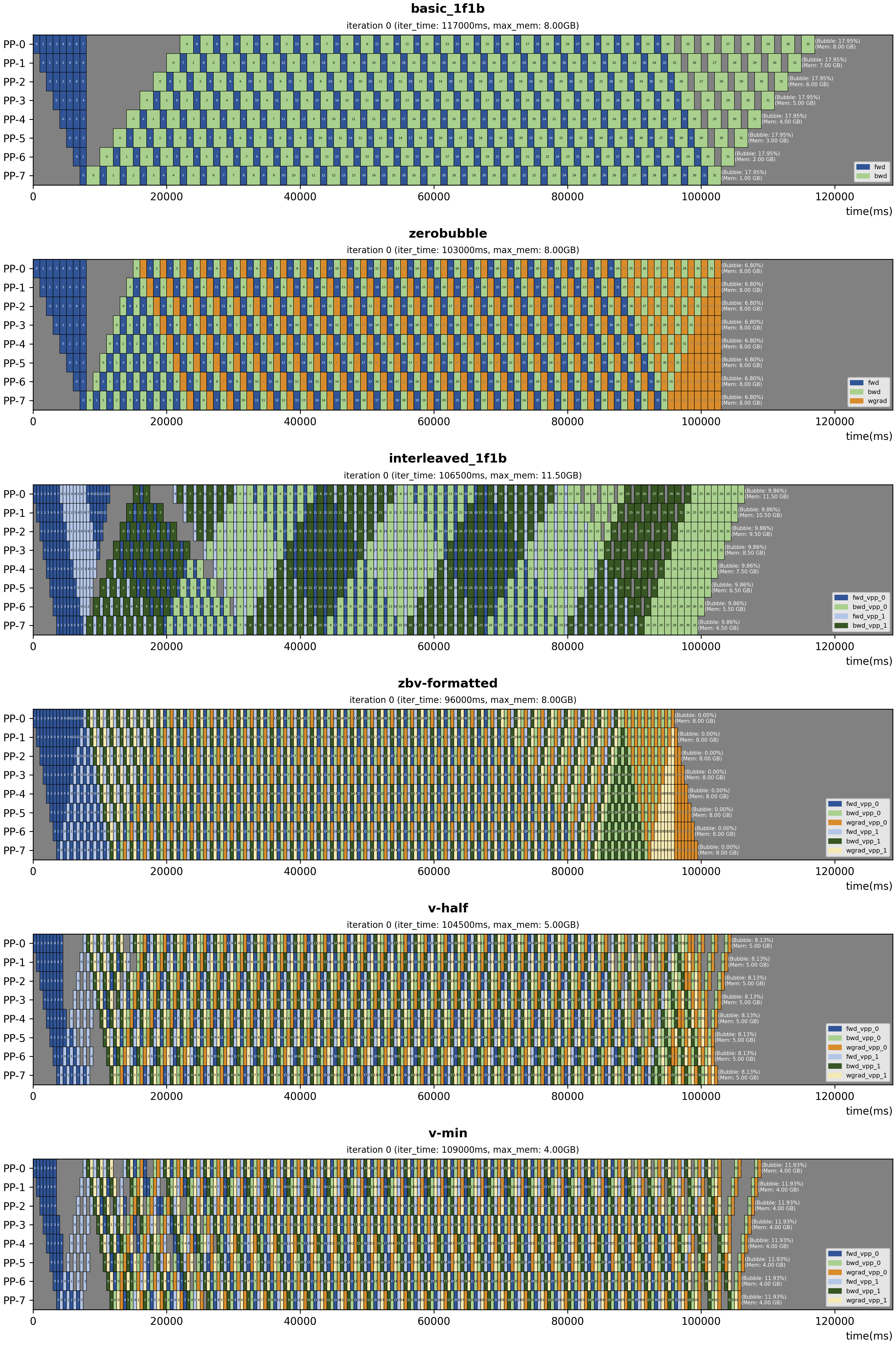
• Simulation perf

After running the simulator with simulator.py, you can visualize the projected schedule using the same configuration YAML. The visualization script generates pipeline schedule diagrams that illustrate the execution timeline of each pipeline stage, making it easy to compare bubble patterns and stage utilization across algorithms.

Run the following command to produce the schedule figures:

python3 tools/visualization/pp_vis/vis.py --config=primus/core/projection/configs/pp_simulation.yaml

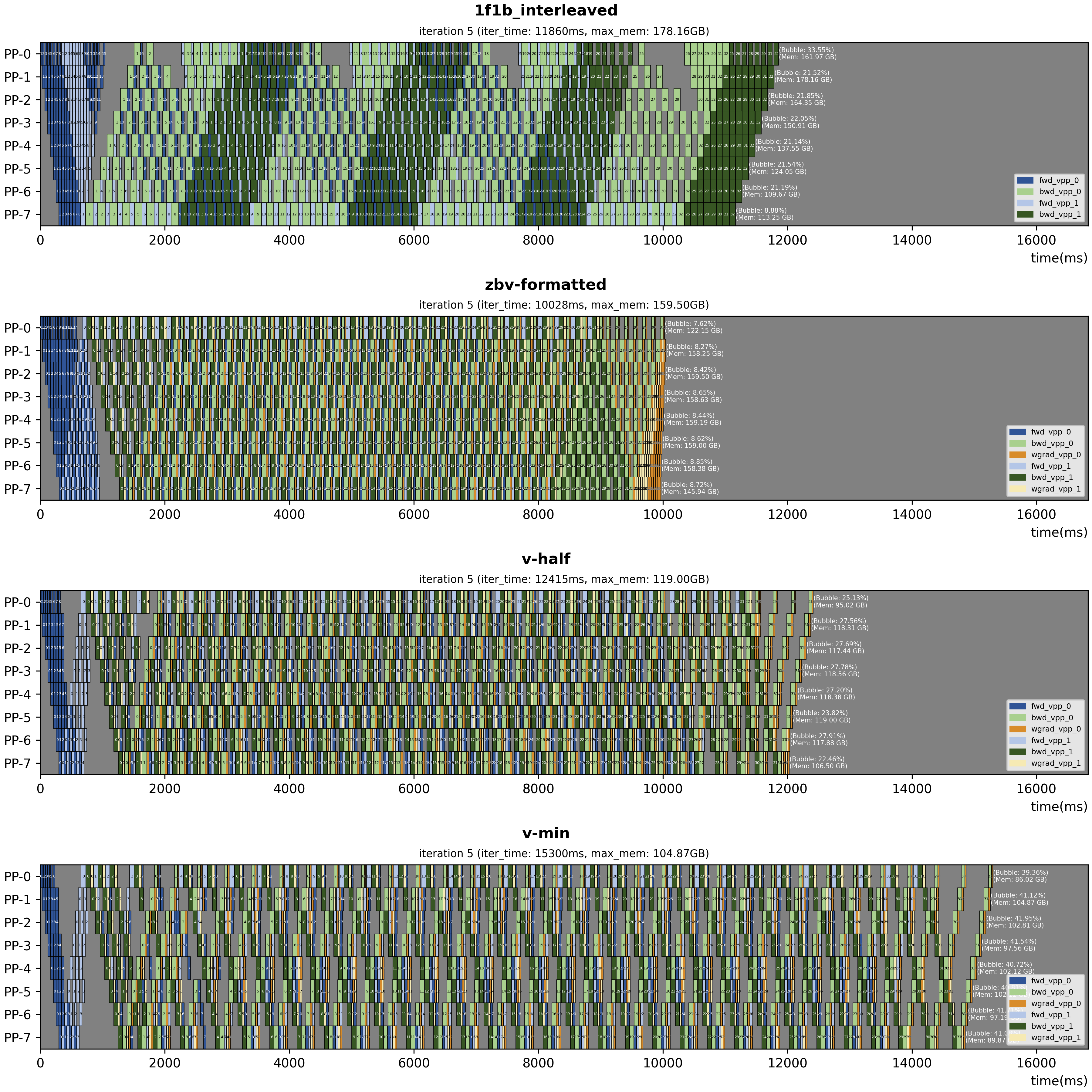
• Real training perf

To visualize schedules from actual training runs, enable the flag dump_pp_config: true in Primus. This produces a directory of per-stage performance data (default: output/pp_data). You can change the output directory via the environment variable DUMP_PP_DIR. Then, set your perf data directory in the draw_from_task_list() function in vis.py and run the script below to generate the pipeline schedule figures.

python3 tools/visualization/pp_vis/vis.py

Run with Megatron-LM Backend

Most configs for using Primus-Pipeline are defined in primus_pipeline.yaml. Two key configs are patch_primus_pipeline, which enables the Primus-Pipeline implementation to replace the original schedule logic in Megatron, and pp_algorithm, which specifies the PP scheduling algorithm to use.

Additionally, some configurations conflict with Primus-pipeline and need to be configured as listed below.

overlap_grad_reduce: false
overlap_param_gather: false
no_persist_layer_norm: true
create_attention_mask_in_dataloader: false
gradient_accumulation_fusion: true

PP schedule algorithm comparison

Our implementation primarily focuses on the zero-bubble family proposed by Sea AI Lab, including zerobubble/zbv/v-half/v-min. Note that post-validation is not currently supported, as it requires substantial optimizer modifications that are challenging to maintain across Megatron-LM versions.

The following table compares different PP scheduling algorithms under the assumption that forward, backward, and weight-grad operations have equal execution time:

Algorithm	VPP size	Bubble Rate	Max Activation Memory	Communication Volume
1f1b	1	(p - 1) / (m + p -1)	p	1
1f1b-interleaved	N	(p - 1) / (m * N + p - 1)	p + (p - 1) / p	N
ZeroBubble(ZB1P)	1	(p - 1) / (3 * (m + p - 1))	p	1
ZBV-formatted	2	(p - 1) / (p - 1 + 6 * m)	p	2
V-half	2	-	p / 2 + x	2
V-min	2	-	p / 3 + x	2

Note: V-half and V-min employ greedy algorithms and therefore lack closed-form bubble-rate formulas. Use the simulator to estimate their bubble rates.

Notation:

• p: number of pipeline stages

• m: number of mini-batches

• x: constant term

Experiments

We ran experiments to validate Primus-Pipeline performance. This section reports results for two setups: Llama2-7B on 1 node with PP8, and the Qwen3-235B MoE model with PP4 and EP8.

Llama2-7B verification

• Setup: MI300 cluster, 1 node, PP8, Llama2-7B model

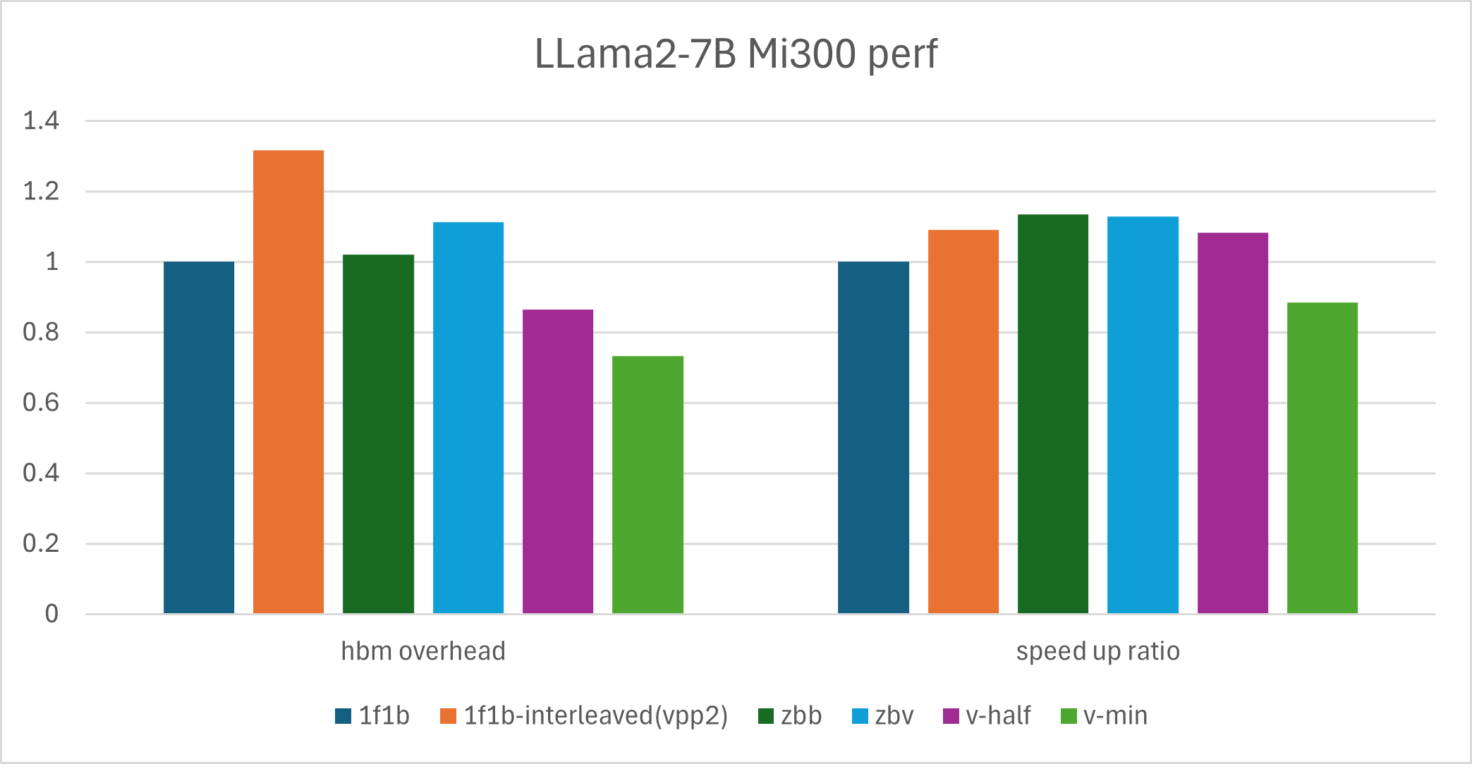
The table below compares different PP algorithms with 8 pipeline stages on Llama2-7B. This dense (non-MoE) model serves as a quick reference for how each algorithm trades off throughput (TFLOPS, tokens/s/device) and memory (max_memory, max_mem_percent).

PP	VPP	PP-algorithm	tokens/s/device	TFLOPS	max_memory	max_mem_percent	HBM overhead	speed up ratio
8	1	1f1b	10057	235.7	16.26	8.47%	1	1
8	2	1f1b-interleaved(vpp2)	10974	257.3	21.40	11.15%	1.31	1.09
8	2	zbb	11411	268	16.59	8.64%	1.02	1.13
8	2	zbv	11347	265.9	18.11	9.43%	1.11	1.12
8	2	v-half	10894	255.1	14.06	7.32%	0.86	1.08
8	2	v-min	8897.2	208.5	11.90	6.20%	0.73	0.88

The bar chart below provides a clearer comparison of memory and throughput among different algorithms on the Llama2-7B model.

Qwen3-235B verification

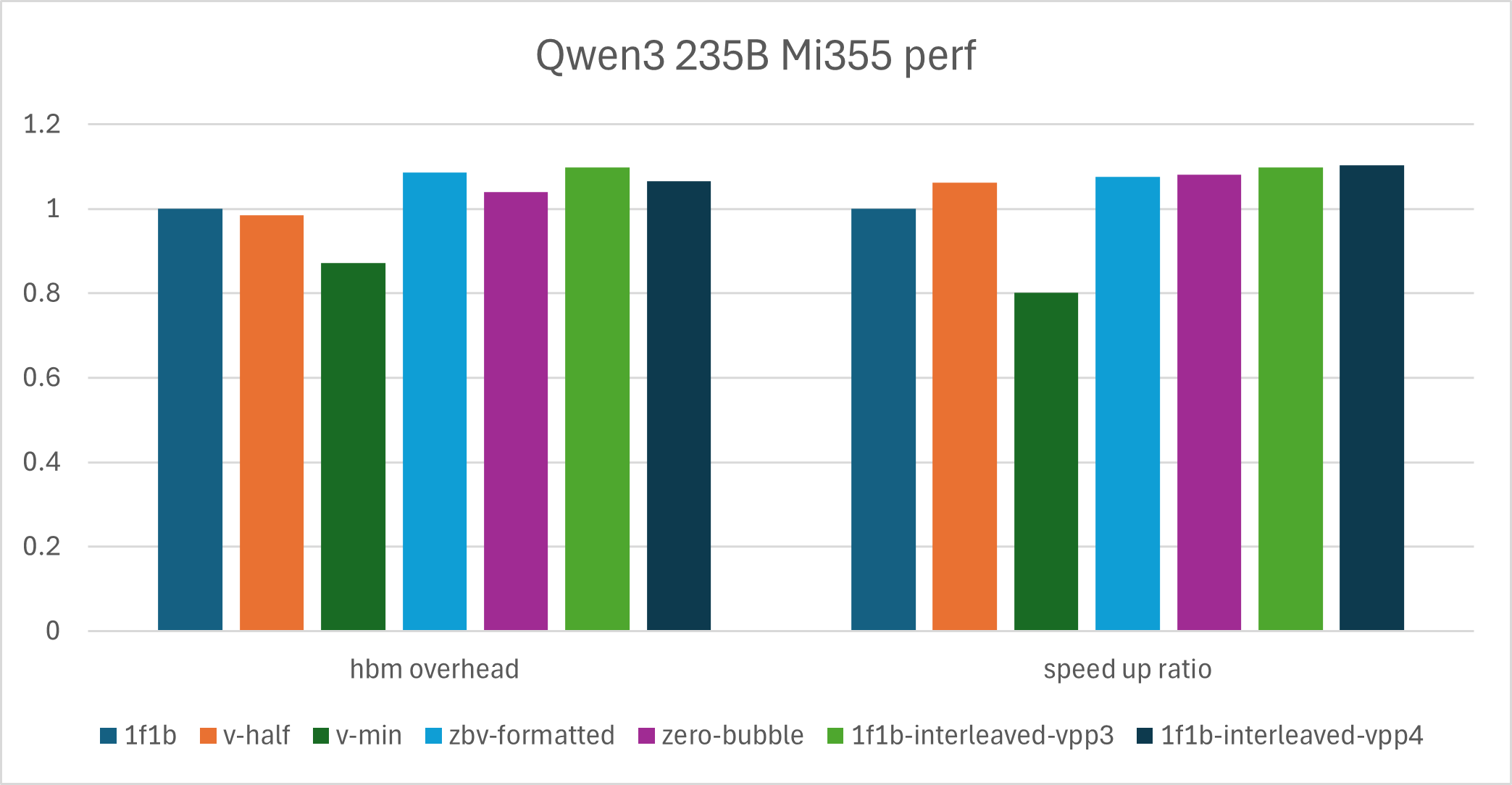
• Setup: MI355 cluster, 4 nodes, PP4, EP8, Qwen3-235B model

We use Qwen3-235B to illustrate large-scale MoE training in practice. For this setup, zero-bubble–style algorithms are not always the top choice for peak throughput but remain a good option when reducing memory usage is important.

PP	VPP	PP-algorithm	tokens/s/device	TFLOPS	max_memory	max_mem_percent	HBM overhead	speed up ratio
4	1	1f1b	2742.4	406	261.58	90.83%	1	1
4	2	v-half	2912.9	431.2	257.84	89.53%	0.98	1.06
4	2	v-min	2200.6	325.8	228.28	79.27%	0.87	0.80
4	2	zbv-formatted	2952.7	437.1	284.36	98.74%	1.09	1.08
4	1	zero-bubble	2963.1	438.6	272.13	94.50%	1.04	1.08
4	3	1f1b-interleaved-vpp2	OOM
4	3	1f1b-interleaved-vpp3	3012.1	445.9	287.13	99.70%	1.10	1.10
4	4	1f1b-interleaved-vpp4	3024.5	447.7	278.82	96.82%	1.06	1.10

We also provide a bar chart for the performance comparison of the Qwen3-235B model.

Best Practice Guide

Based on the results above, we draw the following conclusions.

• Llama-based models show higher throughput and memory gains than MoE models, because the overall network has a larger GEMM footprint and higher activation memory usage.

• For large MoE cases in practice, 1f1b-interleaved reaches a higher throughput roofline than zero-bubble schedules, but it is harder to reduce memory usage. In memory-limited scenarios, v-half is a reasonable option.

Based on these conclusions, we recommend using zero-bubble based algorithms (zero-bubble / zbv / v-half / v-min) instead of 1f1b-interleaved in the following cases:

• A large share of GEMM / Grouped GEMM in the model: dense-layer-heavy models benefit more from splitting weight-grad and input-grad computation. An imbalance in time between the two phases tends to introduce extra bubbles.

• Memory is the bottleneck: 1f1b-interleaved offers limited ways to reduce memory consumption, while v-half and v-min provide practical options when memory is tight.

• Communication is inefficient: 1f1b-interleaved trades extra communication for lower bubble rates, and larger VPP increases communication volume. In most cases, p2p communication can be hidden by overlapping computation, but without AINIC or RDMA support, zbv/v-half/v-min have clearer advantages.

• Extreme partitioning limits: when the model cannot be split beyond VPP rank 2, zbv/v-half/v-min usually outperform 1f1b-interleaved.

Summary

In this blog you will learn how to use Primus-Pipeline, a novel pipeline parallelism framework in Primus. It will helps you investigate and research on PP algorithm in a more flexible way. Below are several ongoing and planned areas of exploration. We welcome contributions, feedback, and new ideas from the community.

1. CPU offloading: Based on the schedule node design, it is easy to control offloading/reloading timing for different mini-batches and model layers. We are adding offload logic to zbv/v-half/v-min algorithms.

2. More algorithms: Implement more state-of-the-art PP schedules like Dual-Pipe-V and investigate more efficient PP algorithms. Contributions are welcome.

3. Fine-grained overlap: In technical reports like DeepSeek-V3, PP schedules combine forward and backward passes of different mini-batches and overlap computation and communication. We plan to explore similar fine-grained overlap strategies.

Acknowledgments

We would like to express our sincere gratitude to the SeaAI Lab team and individuals for their invaluable contributions and collaboration, their expertise and support have been instrumental in advancing the progress of this project.

Additional Resources

• zero-bubble-pipeline-parallelism: A set of state-of-the-art PP schedule algorithms implemented based on Megatron-LM.

• Megatron-LM: Widely used framework for large-scale Transformer model training.

• Llama-2-7B: Meta’s Llama 2 7B model used for experimental validation.

• Qwen3-235B: Qwen 235B MoE model used for large-scale experiments.

Disclaimers

Third-party content is licensed to you directly by the third party that owns the content and is not licensed to you by AMD. ALL LINKED THIRD-PARTY CONTENT IS PROVIDED “AS IS” WITHOUT A WARRANTY OF ANY KIND. USE OF SUCH THIRD-PARTY CONTENT IS DONE AT YOUR SOLE DISCRETION AND UNDER NO CIRCUMSTANCES WILL AMD BE LIABLE TO YOU FOR ANY THIRD-PARTY CONTENT. YOU ASSUME ALL RISK AND ARE SOLELY RESPONSIBLE FOR ANY DAMAGES THAT MAY ARISE FROM YOUR USE OF THIRD-PARTY CONTENT.