A Guide to Implementing and Training Generative Pre-trained Transformers (GPT) in JAX on AMD GPUs

2 July, 2024 by Douglas Jia.

In this blog, we illustrate the process of implementing and training a Generative Pre-trained Transformer (GPT) model in JAX, drawing from Andrej Karpathy’s PyTorch-based nanoGPT. Through an examination of the distinctions between PyTorch and JAX in realizing key components of the GPT model—such as self-attention and optimizers—we elucidate the distinctive attributes of JAX. Moreover, we offer an introductory overview of GPT model fundamentals to enhance comprehension.

Background

In the realm of data science and machine learning, the choice of framework plays a crucial role in model development and performance. PyTorch has long been favored by researchers and practitioners for its intuitive interface and dynamic computation graph. On the other hand, JAX/Flax offers a unique approach with its focus on functional programming and composable function transformations. JAX, developed by Google, provides automatic differentiation and composable function transformations for Python and NumPy code. Flax, built on top of JAX, offers a high-level API for defining and training neural network models while harnessing the power of JAX for automatic differentiation and hardware acceleration. It aims to provide flexibility and ease of use with features like modular model construction and support for distributed training. While PyTorch excels in flexibility, JAX stands out for performance optimization and hardware acceleration, particularly on GPUs and TPUs. Additionally, JAX simplifies device management by transparently running on available accelerators without explicit device specification.

Andrej Karpathy developed nanoGPT as a streamlined rendition of the GPT language model, a transformative deep learning architecture in natural language processing. Unlike the resource-intensive GPT models from OpenAI, nanoGPT is engineered to be lightweight and easily deployable, even on modest hardware setups. Despite its compact size, nanoGPT preserves the core functionalities of the GPT model, including text generation, language comprehension, and adaptability to various downstream applications. Its significance lies in democratizing access to cutting-edge language models, empowering researchers, developers, and enthusiasts to delve into natural language AI even with consumer GPUs.

In this blog, we’ll walk through the process of converting PyTorch-defined GPT models and training procedures to JAX/Flax, using nanoGPT as our guiding example. By dissecting the disparities between these frameworks in implementing crucial GPT model components and training mechanisms such as self-attention and optimizers, our aim is to furnish a comprehensive comparative guide for mastering JAX. Additionally, we offer a foundation for crafting personalized JAX models and training frameworks by adapting our JAX nanoGPT code. This endeavor enhances the model’s flexibility and deployment ease, fostering wider adoption and progression of ML based NLP technologies. In the final section of this blog, we will demonstrate how to pre-train the nanoGPT-JAX model using the character-level Shakespeare dataset and generate sample outputs.

If you’re an experienced developer familiar with JAX/Flax and seeking implementation details to aid your project, you can directly access all our source code on the rocm-blogs GitHub page.

Converting PyTorch model definitions and training procedures to JAX

To train and execute a deep learning model, including LLMs, two essential files are typically required on a high level: model.py and train.py. In the context of a GPT model, the model.py file defines the architecture, encompassing crucial components such as:

• Token and position embedding layers;

• Multiple blocks where each block consists of an attention layer and a multilayer perceptron (MLP) layer, each preceded by a normalization layer to standardize the input along the sequence dimension;

• A final linear layer which is typically called the language model head and is responsible for mapping the transformer model’s output to a vocabulary distribution.

The train.py file outlines the training procedures. It incorporates essential components such as:

• The data loader, which is responsible for sequentially supplying randomly sampled data batches during training iterations;

• The optimizer, which dictates parameter updates.

• A training state, which is unique to Flax. It is responsible for managing and updating model parameters, alongside other components such as the optimizer and forward pass. It’s crucial to note that while Flax integrates these components into a unified training state, PyTorch handles them separately within the training loop.

In this section, we’ll guide you through the process of converting key components of the nanoGPT model and training procedures from PyTorch to JAX. We’ll present PyTorch and JAX code modules side by side for convenient comparison. Please note that the code snippets in this section are for illustrative purposes only. They are not executable, as we’ve omitted essential code necessary for execution but less relevant to the topic (e.g., module imports). Please refer to the model.py and train.py files in our GitHub repository for the complete implementation.

Self attention

The self-attention module in a GPT model weighs the importance of words in a sequence by computing attention scores based on their relationships with other words. This enables effective capture of long-range dependencies and contextual information, essential for tasks like natural language understanding and generation.

To illustrate the difference between PyTorch and JAX implementation of the self-attention module, we include the corresponding code blocks below.

PyTorch

JAX/Flax

class CausalSelfAttention(nn.Module): def __init__(self, config): super().__init__() assert config.n_embd % config.n_head == 0 # key, query, value projections for all heads, but in a batch self.c_attn = nn.Linear(config.n_embd, 3 * config.n_embd, bias=config.bias) # output projection self.c_proj = nn.Linear(config.n_embd, config.n_embd, bias=config.bias) # regularization self.attn_dropout = nn.Dropout(config.dropout) self.resid_dropout = nn.Dropout(config.dropout) self.n_head = config.n_head self.n_embd = config.n_embd self.dropout = config.dropout # flash attention make GPU go brrrrr but support is only # in PyTorch >= 2.0 self.flash = hasattr(torch.nn.functional, "scaled_dot_product_attention") if not self.flash: print( "WARNING: using slow attention. Flash Attention \ requires PyTorch >= 2.0" ) # causal mask to ensure that attention is only applied to # the left in the input sequence self.register_buffer( "bias", torch.tril(torch.ones(config.block_size, config.block_size)).view( 1, 1, config.block_size, config.block_size ), ) def forward(self, x): # batch size, sequence length, embedding dimension (n_embd) (B, T, C,) = x.size() # calculate query, key, values for all heads in batch and # move head forward to be the batch dim q, k, v = self.c_attn(x).split(self.n_embd, dim=2) k = k.view(B, T, self.n_head, C // self.n_head).transpose( 1, 2 ) # (B, nh, T, hs) q = q.view(B, T, self.n_head, C // self.n_head).transpose( 1, 2 ) # (B, nh, T, hs) v = v.view(B, T, self.n_head, C // self.n_head).transpose( 1, 2 ) # (B, nh, T, hs) # causal self-attention; Self-attend: (B, nh, T, hs) x # (B, nh, hs, T) -> (B, nh, T, T) if self.flash: # efficient attention using Flash Attention CUDA kernels y = torch.nn.functional.scaled_dot_product_attention( q, k, v, attn_mask=None, dropout_p=self.dropout if self.training else 0, is_causal=True, ) else: # manual implementation of attention att = (q @ k.transpose(-2, -1)) * (1.0 / math.sqrt(k.size(-1))) att = att.masked_fill(self.bias[:, :, :T, :T] == 0, float("-inf")) att = F.softmax(att, dim=-1) att = self.attn_dropout(att) # (B, nh, T, T) x (B, nh, T, hs) -> (B, nh, T, hs) y = att @ v y = ( y.transpose(1, 2).contiguous().view(B, T, C) ) # re-assemble all head outputs side by side # output projection y = self.resid_dropout(self.c_proj(y)) return y

class CausalSelfAttention(nn.Module): #GPTConfig is a class that defines the model architecture, including parameters such as vocabulary size, block size (length of the context window), number of attention heads, embedding dimension, and more. For detailed information, refer to the GPTConfig class definition in the model.py file. config: GPTConfig @nn.compact def __call__(self, x, train=False, rng1=None, rng2=None): assert self.config.n_embd % self.config.n_head == 0 # batch size, sequence length, embedding dimension (n_embd) (B, T, C,) = x.shape # calculate query, key, values for all heads in batch and # move head forward to be the batch dim q, k, v = jnp.split( nn.Dense(self.config.n_embd * 3, name="c_attn")(x), 3, axis=-1 ) k = k.reshape(B, T, self.config.n_head, C // self.config.n_head).swapaxes( 1, 2 ) # (B, nh, T, hs) q = q.reshape(B, T, self.config.n_head, C // self.config.n_head).swapaxes( 1, 2 ) # (B, nh, T, hs) v = v.reshape(B, T, self.config.n_head, C // self.config.n_head).swapaxes( 1, 2 ) # (B, nh, T, hs) att = ( jnp.einsum("bhts,bhqs->bhtq", q, k, optimize=True) if self.config.use_einsum else jnp.matmul(q, k.swapaxes(-2, -1)) ) * (1.0 / jnp.sqrt(k.shape[-1])) mask = jnp.tril(jnp.ones((T, T))).reshape((1, 1, T, T)) att = jnp.where(mask == 0, float("-inf"), att) att = nn.softmax(att, axis=-1) att = nn.Dropout( self.config.dropout, name="attn_dropout", deterministic=not train )(att, rng=rng1) y = ( jnp.einsum("bhts,bhsq->bhtq", att, v, optimize=True) if self.config.use_einsum else jnp.matmul(att, v) ) # (B, nh, T, T) x (B, nh, T, hs) -> (B, nh, T, hs) y = y.swapaxes(1, 2).reshape( B, T, C ) # re-assemble all head outputs side by side # output projection y = nn.Dense(self.config.n_embd, name="c_proj")(y) y = nn.Dropout( self.config.dropout, name="resid_dropout", deterministic=not train )(y, rng=rng2) return y

In the side-by-side comparison above, you’ll notice that in the CausalSelfAttention class, PyTorch requires an __init__ method to initialize all layers and a forward method to define the computations, commonly known as the “forward pass.” In contrast, Flax offers a more concise approach: you can utilize the @nn.compact decorated __call__ method to initialize the layers inline and define the computations simultaneously. This results in a significantly shorter and more concise implementation in JAX/Flax compared to PyTorch.

To facilitate a smoother migration from PyTorch to JAX/Flax, Flax introduces the setup method, which serves as the equivalent of __init__. With setup, you can initialize all layers and use the __call__ method (without the @nn.compact decorator) to perform the forward pass. This methodology will be demonstrated when defining the GPT class below. Please note that the behavior of nn.compact isn’t different from using the setup function; it is merely a matter of personal preference.

Another notable difference is that while PyTorch requires specifying both input and output shapes for layers, Flax only requires specifying the output shape, as it can infer the input shape based on the provided input. This feature is particularly useful when the shapes of the inputs are either unknown or difficult to determine during initialization.

Defining the GPT model

Once the CausalSelfAttention class is defined, we’ll proceed to define the MLP class and combine these two classes into a Block class. Subsequently, within the primary GPT class, we’ll integrate all these elements—embedding layers, blocks comprising attention and MLP layers, and the language model head—to construct the GPT model. Notably, the Block layer architecture will be repeated n_layer times in the GPT model. This repetition facilitates hierarchical feature learning, enabling the model to capture various aspects of the input data at different levels of abstraction, and progressively capturing more intricate patterns and dependencies.

PyTorch

JAX/Flax

class MLP(nn.Module): def __init__(self, config): super().__init__() self.c_fc = nn.Linear(config.n_embd, 4 * config.n_embd, bias=config.bias) self.gelu = nn.GELU() self.c_proj = nn.Linear(4 * config.n_embd, config.n_embd, bias=config.bias) self.dropout = nn.Dropout(config.dropout) def forward(self, x): x = self.c_fc(x) x = self.gelu(x) x = self.c_proj(x) x = self.dropout(x) return x class Block(nn.Module): def __init__(self, config): super().__init__() self.ln_1 = LayerNorm(config.n_embd, bias=config.bias) self.attn = CausalSelfAttention(config) self.ln_2 = LayerNorm(config.n_embd, bias=config.bias) self.mlp = MLP(config) def forward(self, x): x = x + self.attn(self.ln_1(x)) x = x + self.mlp(self.ln_2(x)) return x class GPT(nn.Module): def __init__(self, config): super().__init__() assert config.vocab_size is not None assert config.block_size is not None self.config = config self.transformer = nn.ModuleDict( dict( wte=nn.Embedding(config.vocab_size, config.n_embd), wpe=nn.Embedding(config.block_size, config.n_embd), drop=nn.Dropout(config.dropout), h=nn.ModuleList([Block(config) for _ in range(config.n_layer)]), ln_f=LayerNorm(config.n_embd, bias=config.bias), ) ) self.lm_head = nn.Linear(config.n_embd, config.vocab_size, bias=False) self.transformer.wte.weight = self.lm_head.weight # init all weights self.apply(self._init_weights) # apply special scaled init to the residual projections, per GPT-2 paper for pn, p in self.named_parameters(): if pn.endswith("c_proj.weight"): torch.nn.init.normal_( p, mean=0.0, std=0.02 / math.sqrt(2 * config.n_layer) ) # report number of parameters print("number of parameters: %.2fM" % (self.get_num_params() / 1e6,)) def forward(self, idx, targets=None): device = idx.device b, t = idx.size() assert ( t <= self.config.block_size ), f"Cannot forward sequence of length {t}, block size is only { self.config.block_size}" pos = torch.arange(0, t, dtype=torch.long, device=device) # shape (t) # forward the GPT model itself tok_emb = self.transformer.wte(idx) # token embd shape (b, t, n_embd) pos_emb = self.transformer.wpe(pos) # position embd shape (t, n_embd) x = self.transformer.drop(tok_emb + pos_emb) for block in self.transformer.h: x = block(x) x = self.transformer.ln_f(x) if targets is not None: # if we are given some desired targets also calculate the loss logits = self.lm_head(x) loss = F.cross_entropy( logits.view(-1, logits.size(-1)), targets.view(-1), ignore_index=-1 ) else: # inference-time mini-optimization: only forward the lm_head on the # very last position logits = self.lm_head( x[:, [-1], :] ) # note: using list [-1] to preserve the time dim loss = None return logits, loss

class MLP(nn.Module): config: GPTConfig @nn.compact def __call__(self, x, train=False, rng=None): x = nn.Dense(4 * self.config.n_embd, use_bias=self.config.bias)(x) x = nn.gelu(x) x = nn.Dense(self.config.n_embd, use_bias=self.config.bias)(x) x = nn.Dropout(self.config.dropout, deterministic=not train)(x, rng=rng) return x class Block(nn.Module): config: GPTConfig @nn.compact def __call__(self, x, train=False, rng1=None, rng2=None, rng3=None): x = x + CausalSelfAttention(self.config, name="attn")( nn.LayerNorm(use_bias=self.config.bias, name="ln_1")(x), train=train, rng1=rng1, rng2=rng2, ) x = x + MLP(self.config, name="mlp")( nn.LayerNorm(use_bias=self.config.bias, name="ln_2")(x), train=train, rng=rng3, ) return x class GPT(nn.Module): config: GPTConfig def setup(self): assert self.config.vocab_size is not None assert self.config.block_size is not None self.wte = nn.Embed(self.config.vocab_size, self.config.n_embd) self.wpe = nn.Embed(self.config.block_size, self.config.n_embd) self.drop = nn.Dropout(self.config.dropout) self.h = [Block(self.config) for _ in range(self.config.n_layer)] self.ln_f = nn.LayerNorm(use_bias=self.config.bias) def __call__(self, idx, targets=None, train=False, rng=jax.random.key(0)): _, t = idx.shape assert ( t <= self.config.block_size ), f"Cannot forward sequence of length {t}, block size is only { self.config.block_size}" pos = jnp.arange(t, dtype=jnp.int32) # forward the GPT model itself tok_emb = self.wte(idx) # token embeddings of shape (b, t, n_embd) pos_emb = self.wpe(pos) # position embeddings of shape (t, n_embd) rng0, rng1, rng2, rng3 = jax.random.split(rng, 4) x = self.drop(tok_emb + pos_emb, deterministic=False, rng=rng0) for block in self.h: x = block(x, train=train, rng1=rng1, rng2=rng2, rng3=rng3) x = self.ln_f(x) if targets is not None: # weight tying (https://github.com/google/flax/discussions/2186) logits = self.wte.attend( x ) # (b, t, vocab_size) loss = optax.softmax_cross_entropy_with_integer_labels( logits, targets ).mean() else: logits = self.wte.attend(x[:, -1:, :]) loss = None return logits, loss

In the JAX/Flax implementation provided above, you’ll notice that we utilized the @nn.compact decorator to consolidate the initialization and forward pass within the __call__ method for both the MLP and Block classes. However, we opted to separate the initialization process using the setup method and the forward pass using the __call__ method in the GPT class. One notable distinction between PyTorch and Flax lies in the specification of weight tying, which involves sharing weights between the embedding layer and the output layer (language model head). This practice is beneficial as both matrices often capture similar semantic properties. In PyTorch, weight tying is accomplished using self.transformer.wte.weight = self.lm_head.weight, while Flax achieves this using the self.wte.attend method. Additionally, in JAX, it’s necessary to explicitly specify a random number generator key when introducing randomness, a step that’s unnecessary in PyTorch.

The optimizer

Optimizers play a crucial role in training deep learning models by defining update rules and strategies for adjusting model parameters. They can also integrate regularization techniques like weight decay to prevent overfitting and enhance generalization.

Some popular optimizers include

• Stochastic Gradient Descent (SGD) with Momentum: This optimizer introduces a momentum term to accelerate parameter updates in the direction of recent gradients.

• Adam: Adam combines the advantages of momentum and root-mean-square (RMS) propagation, dynamically adjusting the learning rate for each parameter based on the moving averages of gradients and squared gradients.

• AdamW: A variant of Adam that incorporates weight decay, often employed in various deep learning tasks.

In training large language models (LLMs), it’s common practice to selectively apply weight decay to layers involved in matrix multiplications (explained by Andrej Karpathy).

In the code examples below, observe how PyTorch and JAX handle weight decay differently due to variations in the data structures used to store parameters. For a deeper understanding, interested readers can explore this tutorial on PyTrees.

PyTorch

JAX/Flax

def configure_optimizers(self, weight_decay, learning_rate, betas, device_type): # start with all of the candidate parameters param_dict = {pn: p for pn, p in self.named_parameters()} # filter out those that do not require grad param_dict = {pn: p for pn, p in param_dict.items() if p.requires_grad} # create optim groups. Any parameters that is 2D will be weight decayed, # otherwise no. I.e. all weight tensors in matmuls + embeddings decay, # all biases and layernorms don't. decay_params = [p for n, p in param_dict.items() if p.dim() >= 2] nodecay_params = [p for n, p in param_dict.items() if p.dim() < 2] optim_groups = [ {"params": decay_params, "weight_decay": weight_decay}, {"params": nodecay_params, "weight_decay": 0.0}, ] # Create AdamW optimizer and use the fused version if it is available fused_available = "fused" in inspect.signature(torch.optim.AdamW).parameters use_fused = fused_available and device_type == "cuda" extra_args = dict(fused=True) if use_fused else dict() optimizer = torch.optim.AdamW( optim_groups, lr=learning_rate, betas=betas, **extra_args ) print(f"using fused AdamW: {use_fused}") return optimizer

def configure_optimizers(self, params, weight_decay, learning_rate, betas): # Only implement weight decay on weights that are involved in matmul. label_fn = ( lambda path, value: "no_decay" if (value.ndim < 2) or ("embedding" in path) else "decay" ) # Create optimization groups decay_opt = optax.adamw( learning_rate, weight_decay=weight_decay, b1=betas[0], b2=betas[1] ) nodecay_opt = optax.adam(learning_rate, b1=betas[0], b2=betas[1]) tx = optax.multi_transform( {"decay": decay_opt, "no_decay": nodecay_opt}, flax.traverse_util.path_aware_map(label_fn, params), ) return tx

The training loop

The training loop entails the iterative process of training a model on a dataset, involving these steps:

1. Data Loading: Batching training data, often text sequences, from a dataset using a data loader function.

2. Forward Pass: Propagating input sequences through the model to generate predictions.

3. Loss Calculation: Determining the loss between model predictions and actual targets (e.g., the next word in a sequence).

4. Backward Pass (Gradient Calculation): Computing gradients of the loss with respect to model parameters through backpropagation.

5. Parameter Update: Adjusting model parameters using an optimizer based on computed gradients.

6. Repeat: Repeating steps 2-5.

The training loop aims to minimize the loss function and optimize model parameters for accurate predictions on unseen data. In this section, we solely present the JAX/Flax implementation, utilizing a unified training state class to store the model, parameters, and optimizer, performing essential steps like forward pass and parameter update. The JAX approach significantly differs from PyTorch’s design, thus a direct side-by-side comparison may not be beneficial. Those interested can conduct their own comparison with the PyTorch implementation.

The train state

In the code block below, you’ll notice that the train_state class of variable state contains the model’s forward pass definition, optimizer, and parameters. What sets Flax apart from PyTorch is that the model and parameters are separated into two variables. To initialize the parameters, you must provide some sample data to the defined model, allowing the layers’ shapes to be inferred from this data. Therefore, you can consider the model as a fixed variable defining the forward pass architecture, while you update other variables held by the state, such as parameters and the optimizer, within the training loop.

# Define function to initialize the training state.
def init_train_state(
    model,
    params,
    learning_rate,
    weight_decay=None,
    beta1=None,
    beta2=None,
    decay_lr=True,
    warmup_iters=None,
    lr_decay_iters=None,
    min_lr=None,
) -> train_state.TrainState:
    # learning rate decay scheduler (cosine with warmup)
    if decay_lr:
        assert warmup_iters is not None, "warmup_iters must be provided"
        assert lr_decay_iters is not None, "lr_decay_iters must be provided"
        assert min_lr is not None, "min_lr must be provided"
        assert (
            lr_decay_iters >= warmup_iters
        ), "lr_decay_iters must be greater than or equal to warmup_iters"
        lr_schedule = optax.warmup_cosine_decay_schedule(
            init_value=1e-9,
            peak_value=learning_rate,
            warmup_steps=warmup_iters,
            decay_steps=lr_decay_iters,
            end_value=min_lr,
        )
    else:
        lr_schedule = learning_rate
    # Create the optimizer
    naive_optimizer = model.configure_optimizers(
        params,
        weight_decay=weight_decay,
        learning_rate=lr_schedule,
        betas=(beta1, beta2),
    )
    # Add gradient clipping
    optimizer = optax.chain(optax.clip_by_global_norm(grad_clip), naive_optimizer)
    # Create a State
    return (
        train_state.TrainState.create(
            apply_fn=model.apply, tx=optimizer, params=params
        ),
        lr_schedule,
    )


model = GPT(gptconf)
# idx here is a dummy input used for initializing the parameters
idx = jnp.ones((3, gptconf.block_size), dtype=jnp.int32)
params = model.init(jax.random.PRNGKey(1), idx)
state, lr_schedule = init_train_state(
    model,
    params["params"],
    learning_rate,
    weight_decay,
    beta1,
    beta2,
    decay_lr,
    warmup_iters,
    lr_decay_iters,
    min_lr,
)

The train step

The train_step function orchestrates the backpropagation process, which computes gradients based on the loss from the forward pass and subsequently updates the state variable. It accepts state as an argument and returns the updated state, integrating information from the current batch of data. It’s worth noting that we explicitly provide a random number key rng to the train_step function to ensure the proper functioning of dropout layers.

def loss_fn(params, x, targets=None, train=True, rng=jax.random.key(0)):
    _, loss = state.apply_fn(
        {"params": params}, x, targets=targets, train=train, rng=rng
    )
    return loss

# The function below JIT-compiles the `train_step` function. The `jax.value_and_grad(loss_fn)` creates a function that evaluates both `loss_fn` and its gradient. As a common practice, you only need to JIT-compile the outermost function.
@partial(jax.jit, donate_argnums=(0,))
def train_step(
    state: train_state.TrainState,
    batch: jnp.ndarray,
    rng: jnp.ndarray = jax.random.key(0),
):
    x, y = batch
    key0, key1 = jax.random.split(rng)
    gradient_fn = jax.value_and_grad(loss_fn)
    loss, grads = gradient_fn(state.params, x, targets=y, rng=key0, train=True)
    state = state.apply_gradients(grads=grads)
    return state, loss, key1

The loop

This is the concluding step of the training procedure: defining the training loop. Within this loop, the train_step function will iteratively update the state with new information from each batch of data. The loop will continue until the termination condition is met, such as exceeding the pre-set maximum training iterations.

while True:

    if iter_num == 0 and eval_only:
        break

    state, loss, rng_key = train_step(state, get_batch("train"), rng_key)

    # timing and logging
    t1 = time.time()
    dt = t1 - t0
    t0 = t1
    iter_num += 1

    # termination conditions
    if iter_num > max_iters:
        break

Please note that the actual training loop is more complex than what’s shown above as it typically includes evaluation and checkpointing steps and other logging steps which can be helpful to monitor the training progress and debug. The saved checkpoints can be used for resuming training or making inferences later on. However, we’ll omit these parts due to space constraints in the blog. Interested readers can delve into our source code for further exploration.

Implementation

Now, we’ll guide you through setting up the runtime environment, initiating training and fine-tuning, and generating text using the final trained checkpoints.

Environment setup

We executed the implementation within a PyTorch ROCm 6.1 docker container (check the list of supported OSs and AMD hardware) on an AMD GPU to facilitate a comparison between PyTorch and JAX, given that the original nanoGPT is implemented in PyTorch. We’ll install the necessary packages, including JAX and Jaxlib, on the container. Please note that, although we used an AMD GPU for our blog, our code does not contain any AMD-specific modifications. This highlights the adaptability of ROCm to key deep learning frameworks like PyTorch and JAX.

First, pull and run the docker container with the code below in a Linux shell:

docker run -it --ipc=host --network=host --device=/dev/kfd --device=/dev/dri \
           --group-add video --cap-add=SYS_PTRACE --security-opt seccomp=unconfined \
           --name=nanogpt rocm/pytorch:rocm6.1_ubuntu22.04_py3.10_pytorch_2.1.2 /bin/bash

Next, execute the following code within the docker container to install the necessary Python packages and configure the environment variable for XLA:

python3 -m pip install --upgrade pip
pip install optax==0.2.2 flax==0.8.2 transformers==4.38.2 tiktoken==0.6.0 datasets==2.17.1
python3 -m pip install https://github.com/ROCmSoftwarePlatform/jax/releases/download/jaxlib-v0.4.26/jaxlib-0.4.26+rocm610-cp310-cp310-manylinux2014_x86_64.whl
python3 -m pip install https://github.com/ROCmSoftwarePlatform/jax/archive/refs/tags/jaxlib-v0.4.26.tar.gz
pip install numpy==1.22.0
export XLA_FLAGS="--xla_gpu_autotune_level=0"

Then, download the files used for this blog from the ROCm/rocm-blogs GitHub repository with the command below.

git clone https://github.com/ROCm/rocm-blogs.git
cd rocm-blogs/blogs/artificial-intelligence/nanoGPT-JAX

Ensure that all subsequent operations are performed within the nanoGPT-JAX folder.

Pre-train a nanoGPT model

The original nanoGPT repository provides several dataset processing pipelines for pre-training the GPT model. For instance, you can train a nanoGPT model with the Shakespeare dataset at the character level or train a GPT2 model (or other GPT2 model variants, such as GPT2-medium) with either the Shakespeare or OpenWebText dataset. In this section, we will demonstrate how to implement pre-training and fine-tuning. You can customize the dataset processing pipeline and the config file to use other datasets for pre-training or fine-tuning your model of interest.

# Preprocess the character level Shakespeare dataset
python data/shakespeare_char/prepare.py
# Start the pre-training
# The provided configuration file sets up the training of a miniature character-level GPT model using JAX on an AMD GPU. It specifies model architecture parameters, training settings, evaluation intervals, logging preferences, data handling, and checkpointing details, ensuring a comprehensive yet flexible setup for experimenting with and debugging the model.
python train.py config/train_shakespeare_char.py

After the pre-training begins, you’ll observe output similar to the following. Notice that the loss decreases rapidly within the first few tens of iterations.

Evaluating at iter_num == 0...
step 0: train loss 4.3827, val loss 4.3902; best val loss to now: 4.3902
iter 0: loss 4.4377, time 41624.53ms
iter 10: loss 3.4575, time 92.16ms
iter 20: loss 3.2899, time 88.92ms
iter 30: loss 3.0639, time 84.89ms
iter 40: loss 2.8163, time 85.28ms
iter 50: loss 2.6761, time 86.26ms

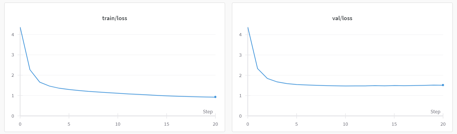
The initial step (iter 0) took considerably longer than subsequent steps. This is because, during the first step, JAX compiles the model and training loop to optimize calculations, enabling faster execution in future iterations. Depending on the hardware you’re using, the pre-training process can take anywhere from several minutes to several tens of minutes to complete. You’ll observe that the best validation loss is typically achieved between 2000 and 3000 iterations. After reaching the best validation loss, the training loss may continue to decrease, but the validation loss might start to increase. This phenomenon is known as overfitting. We showed an example train and validation loss plot in the figure above.

Fine-tune a GPT2-medium model

You can also fine-tune a GPT2 model to leverage pre-trained model weights for generating Shakespeare-style text. This means we will use the same Shakespeare dataset but use the GPT2 model architecture instead of the nanoGPT architecture. In the example below, we fine-tuned the gpt2-medium model.

# Preprocess the Shakespeare dataset
python data/shakespeare/prepare.py
# Start the fine-tuning
python train.py config/finetune_shakespeare.py

In the initial iterations, the generated output will resemble the following:

Evaluting at iter_num == 0...
step 0: train loss 3.6978, val loss 3.5344; best val loss to now: 3.5344
iter 0: loss 4.8762, time 74683.51ms
iter 5: loss 4.9065, time 211.08ms
iter 10: loss 4.4118, time 250.01ms
iter 15: loss 4.9343, time 238.35ms

The loss curve shown below clearly indicates overfitting on the validation data.

Generating Samples from Saved Checkpoints

Now that we have obtained the checkpoints for both the pre-trained character-level nanoGPT model and the fine-tuned GPT2-medium model, we can proceed to generate some samples from these checkpoints. We will utilize the sample.py file to generate three samples with “\n” (new line) as the prompt. Feel free to experiment with other prompts as well.

# Generating samples from the character level nanoGPT model
python sample.py --out_dir=out-shakespeare-char

Here is the output you will get:

Overriding: out_dir = out-shakespeare-char
Loading meta from data/shakespeare_char/meta.pkl...

Generated output __0__: 
__________________________________

MBRCKaGEMESCRaI:Conuple to die with him.

MERCUTIO:
There's no sentence of him with a more than a right!

MENENIUS:
Ay, sir.

MENENIUS:
I have forgot you to see you.

MENENIUS:
I will keep you how to say how you here, and I say you all.

BENVOLIO:
Here comes you this last.

MERCUTIO:
That will not said the princely prepare in this; but you
will be put to my was to my true; and will think the
true cannot come to this weal of some secret but your conjured: I think
the people of your countrying hat
__________________________________

Generated output __1__: 
__________________________________

BRCAMPSMNLES:
GREGod rathready and throng fools.

ANGELBOLINA:
And then shall not be more than a right!

First Murderer:
No, nor I: if my heart it, my fellows of our common
prison of Servingman:
I think he shall not have been my high to visit or wit.

LEONTES:
It is all the good to part it of my fault:
And this is mine, one but not that I was it.

First Lord:
But 'tis better knowledge, and merely away
good Capulet: were your honour to be here at all the good
And the banished of your country'st s
__________________________________

Generated output __2__: 
__________________________________

SLCCESTEPSErShCnardareRoman:
Nay?

The garden hath aboard to see a fellow. Will you more than warrant!

First Murderer:
No, nor I: if my heart it, my fellows of your time is,
and you joy you how to save your rest life, I know not her;
My lord, I will be consul to Ireland
To give you and be too possible.

Second Murderer:
Ay, the gods the pride peace of Lancaster and Montague.

LADY GREY:
God give him, my lord; my lord.

KING EDWARD IV:
Poor cousin, intercept of the banishment.

HASTINGS:
The tim
__________________________________

Now, let’s generate samples using the fine-tuned GPT2-medium model:

# Generating samples from the fine-tuned GPT2-medium model
python sample.py --out_dir=out-shakespeare --max_new_tokens=60

Here is the output you will get:

Overriding: out_dir = out-shakespeare
Overriding: max_new_tokens = 60
No meta.pkl found, assuming GPT-2 encodings...

Generated output __0__: 
__________________________________


PERDITA:
It took me long to live, to die again, to see't.

DUKE VINCENTIO:
Why, then, that my life is not so dear as it used to be
And what I must do with it now, I know
__________________________________

Generated output __1__: 
__________________________________


RICHARD:
Farewell, Balthasar, my brother, my friend.

BALTHASAR:
My lord!

VIRGILIA:
BALTHASAR,
As fortune please,
You have been a true friend to me.
__________________________________

Generated output __2__: 
__________________________________


JULIET:
O, live, in sweet joy, in the sight of God,
Adonis, a noble man's son,
In all that my queen is,
An immortal king,
As well temperate as temperate!

All:
O Juno
__________________________________

By comparing the outputs from the two checkpoints, we can observe that the character-level nanoGPT model produces text resembling Shakespearean style but often appears nonsensical, whereas the fine-tuned model generates text with improved readability, demonstrating the effectiveness of customizing LLMs for specific use cases by fine-tuning with task specific dataset.

Although this tutorial concludes here, we hope it serves as a launching pad for your exploration into understanding, coding, and experimenting with LLMs in different frameworks like PyTorch and JAX/Flax.

Acknowledgements and license

We extend our heartfelt appreciation to Andrej Karpathy for developing the PyTorch-implemented nanoGPT repository, which laid the foundation for our work. Without his remarkable contribution, our project would not have been possible. In our current work, we re-wrote three files from the original nanoGPT repo: model.py, sample.py, and train.py.

Additionally, we would like to express our gratitude to Cristian Garcia for his nanoGPT-jax repository, which served as a valuable reference for our work.

Disclaimers

Third-party content is licensed to you directly by the third party that owns the content and is not licensed to you by AMD. ALL LINKED THIRD-PARTY CONTENT IS PROVIDED “AS IS” WITHOUT A WARRANTY OF ANY KIND. USE OF SUCH THIRD-PARTY CONTENT IS DONE AT YOUR SOLE DISCRETION AND UNDER NO CIRCUMSTANCES WILL AMD BE LIABLE TO YOU FOR ANY THIRD-PARTY CONTENT. YOU ASSUME ALL RISK AND ARE SOLELY RESPONSIBLE FOR ANY DAMAGES THAT MAY ARISE FROM YOUR USE OF THIRD-PARTY CONTENT.

Mamba on AMD GPUs with ROCm   Accelerating models on ROCm using PyTorch TunableOp