From Naive to Near-Peak: Building High-Performance GEMM Kernels with Gluon

May 22, 2026 by Lixun Zhang, Jason Furmanek, Peng Sun, Emad Barsoum.

6 min read. | 1488 total words.

Software tools & optimizations

AI/ML, Linear Algebra, Performance, Profiling, Optimization, Hardware, Compiler

HPC

On a single MI355, our most-optimized FP16 GEMM kernel runs at 99% MFMA efficiency — the matrix engine sits idle for a handful of cycles per loop. Getting there took ten versions, a regression along the way, and a profiler open for the whole time. This post is a tour of that path: from a 520 TFLOPS naive baseline to a 1489 TFLOPS near-peak kernel (~3× speedup), then the same design carried forward to BF8 (3257 TFLOPS, 99.72%) and MXFP4 (5255 TFLOPS, 92.41%) for low-precision AI workloads.

The companion repository gfx950-gluon-tutorials is the full tutorial; this post is the map. It is for kernel developers, ML compiler engineers, and performance specialists who want to see how a near-peak kernel is constructed step by step on AMD MI350/MI355 GPUs (gfx950, CDNA4). Triton’s strength is hardware-portable productivity; Gluon is the tool when you need to extract every last percent on a target architecture.

Why Another GEMM Tutorial?

This isn’t a replacement for production libraries like hipBLASLt; it’s the path through the bottlenecks those libraries hide. The tutorial does not start with the final kernel — it starts with a simple FP16 GEMM that is correct but far from optimal, then builds performance one measured bottleneck at a time. Each version isolates one idea so readers can connect code structure to hardware behavior.

Three kernels on AMD MI350/MI355 (gfx950, CDNA4) span the data types most relevant to modern AI workloads:

Kernel	Data type	Shape used in the summary	Documented result
a16w16	FP16	4096x4096x8192	1489 TFLOPS, 98.75% MFMA efficiency
a8w8	BF8	4096x4096x16384	3257 TFLOPS, 99.72% MFMA efficiency
a4w4	MXFP4	4096x4096x32768	5255 TFLOPS, 92.41% MFMA efficiency

These numbers reproduce against the tutorial’s pinned ROCm and Triton versions (documented in the disclaimer) and the runners shipped in scripts/run_perf_table.py. The value of the tutorial is not only the final number, but the path from baseline to that number. The bar chart below visualizes that path version by version, with the regression at v6 and the recovery through v7–v9 both visible on the same scale.

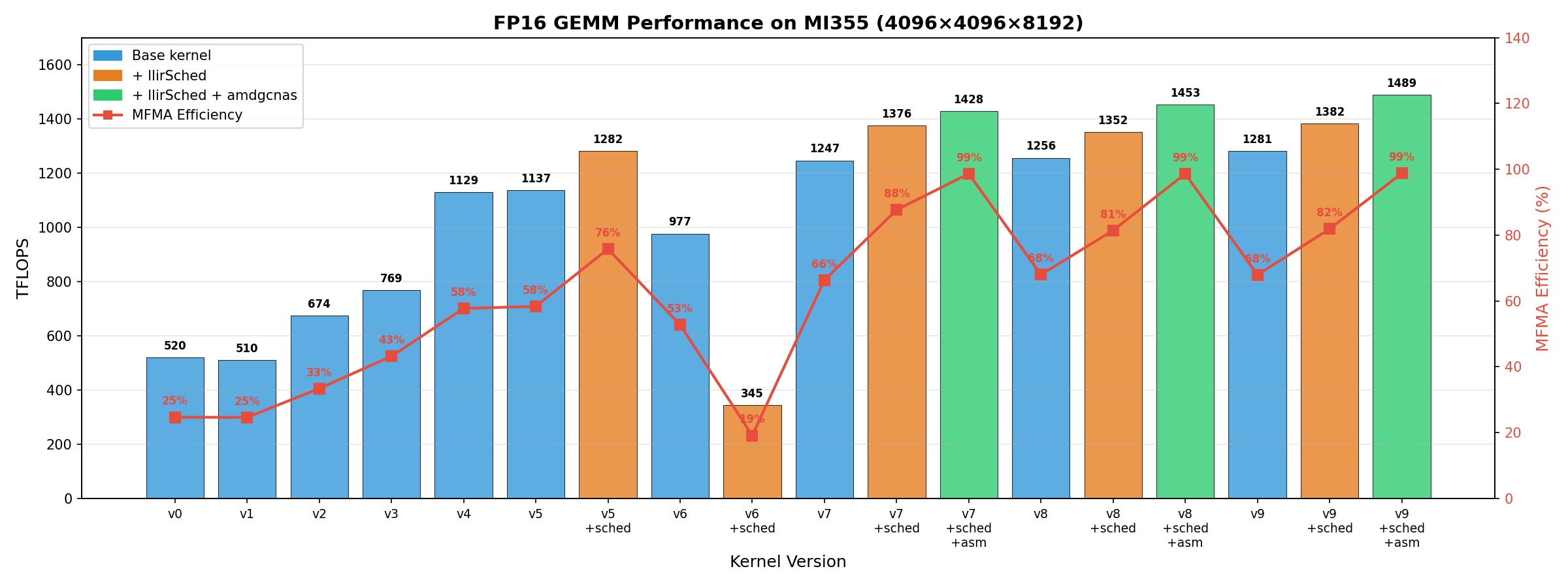
FP16 GEMM performance across the v0–v9 tutorial versions on MI355 (each version shown for the configurations measured for it). Bars are TFLOPS; the red line tracks MFMA efficiency. The visible drop at v6 with llirSched is real — a 73% regression that exposes a register-pressure problem that v7’s slicing then resolves. It is one of the tutorial’s most useful lessons, discussed in Act III. v0 (naive) runs at 520 TFLOPS and 25% MFMA efficiency; v9 (with llirSched and the amdgcnas peephole pass) reaches 1489 TFLOPS and 99% — roughly 2.9× faster than the baseline.

What Gluon Makes Explicit

Gluon is a block-level programming model in Triton. Where conventional thread-level kernels leave the compiler to recover scheduling, register allocation, and memory-movement opportunities from low-level IR, Gluon raises the authoring level to tiles. Layouts are explicit. Pipeline stages are explicit. Register budgeting becomes part of the kernel design, not something discovered after the backend lowers the code. The compiler’s job narrows to faithful lowering and throughput-aware interleaving; the hard problems of traditional GPU compilation (NP-hard scheduling, graph-coloring register allocation) become design problems the kernel author owns.

That explicit control is the central teaching point of the repository. The tutorial repeatedly asks:

• Which instruction should move this data?

• Which layout avoids LDS bank conflicts?

• Which pipeline stage hides global memory or LDS latency?

• How many registers are live at the MFMA boundary?

• What does the trace show after the change?

Hardware reasoning, source code, generated code, and profiler data stay connected throughout.

The FP16 Path: One Bottleneck at a Time

The a16w16 tutorial is the recommended starting point. It is organized as a versioned optimization journey from v0_naive to v9_beyond_hotloop in four acts.

Act I — Getting the basics right (v0–v3). v0_naive establishes a correct FP16 GEMM with explicit layouts. v1_buffer_load switches masked loads to AMD buffer operations so out-of-bounds handling moves into hardware and 140 control-flow branches collapse to 4. v2_async_copy routes data directly from global memory into LDS, eliminating register staging and every ds_write in the inner loop. v3_lds then eliminates LDS bank conflicts by comparing raw, swizzled, and padded shared layouts at the instruction level and picking the one that hits the steady-state ds_read issue rate.

Act II — Hiding latency (v4–v5). v4_global_prefetch adds a two-stage software pipeline so the next K iteration’s data is in flight while the current iteration computes. v5_local_prefetch adds a third stage so MFMA, LDS reads, and global-memory loads can all overlap. At that point instruction ordering becomes a first-class performance problem, so the tutorial introduces llirSched, a Triton-level pass that interleaves MFMA with memory operations according to the hardware throughput model.

Act III — Taming the hardware (v6–v8). This is the act where the tutorial earns its keep — and it does so with a regression.

v6_loop_unroll double-buffers the operand registers so consecutive K iterations swap which register set the MFMA consumes. The per-iteration copy disappears as planned, but TFLOPS crashes to a quarter of v5. The unroll forces both register sets to live concurrently; the working set blows past the 512-VGPR budget and the compiler spills 99 values to scratch on every iteration. Each spill is a scratch_load followed by an s_waitcnt vmcnt(0) that llirSched cannot hide.

The fix isn’t to revert. The right response is to look one layer deeper, identify what changed (here: the live-range overlap that the original copy was silently masking), and resolve that.

v7_sliceN fixes the spill by design — cut the B-tile register footprint in half by computing the output tile in two N-halves rather than one. The live-range overlap dissolves; spills go to zero; v7 + llirSched runs at 87.68% MFMA efficiency, structurally healthy again. This is the most useful lesson in the tutorial: a clean local fix can introduce a regression two layers down, and a methodology — not a hunch — is what stops you from blaming the wrong thing.

The remaining gap from 87.68% to peak is a different problem now that the spills are gone: the register allocator schedules residual AGPR↔VGPR copies inside the loop. amdgcnas (a post-assembly peephole pass over the generated AMDGCN assembly) closes that traffic and brings v7 to 98.65% MFMA efficiency. v8_sliceMN then slices A along M as well, dropping register pressure further and resolving a buffer-load throughput stall that v7 hits at large K. The figure below shows the resulting four-quadrant tile layout.

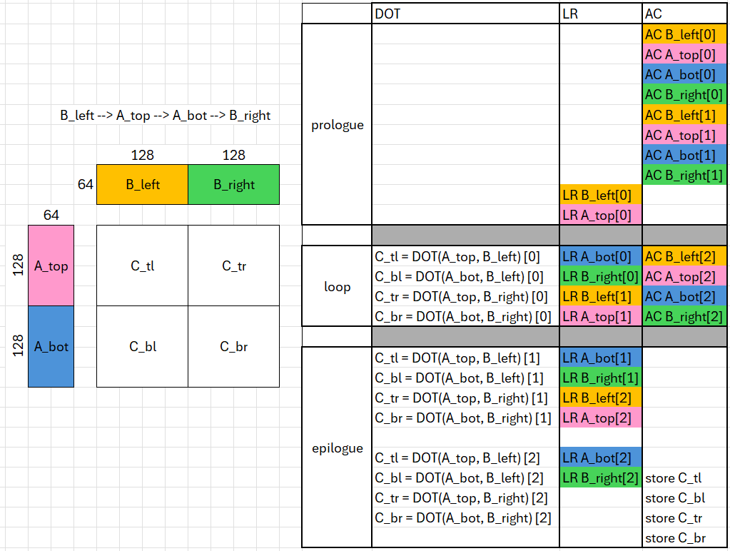
v8 slicing along both M and N. v7 sliced only N (halving the B tile); v8 also slices A along M, dropping register pressure further and structuring the pipeline around four 128×128 quadrants.

Act IV — Beyond the hot loop (v9). With the inner loop already at near-peak MFMA utilization, v9_beyond_hotloop shifts focus to the structural quirk that distinguishes MI350-class hardware: MI350 is a chiplet GPU with 8 XCDs, each carrying its own L2 cache. Workgroups dispatched to different XCDs read from different L2s, so tile pairs that should reuse data instead trigger redundant DRAM traffic — bandwidth and power lost to a hardware structure that doesn’t exist on monolithic dies.

The fix is XCD-aware workgroup remapping plus a GROUP_SIZE_M-based swizzle: assign adjacent tiles to the same XCD so they share L2 lines, then choose the swizzle that minimizes a closed-form objective f(GM) = GM + ⌈P/GM⌉ where P is workgroups per XCD. For P=32, the optimum is GM ∈ {4, 6, 8}. Hardware counters confirm: L2 misses drop from ~5.3M to ~4.1M, power drops with them, and sustained clock — and therefore TFLOPS — lifts the last few percent on top of v8.

This is the kind of insight unique to MI350’s chiplet architecture; it doesn’t transfer from a monolithic-die GPU. The mechanism is unusual; the recipe is open.

Profiling Drives the Tutorial

The tutorial is intentionally measurement-heavy. Instead of treating TFLOPS as the only signal, it tracks the evidence needed to explain a result:

• MFMA efficiency from thread traces

• VGPR usage and spills

• generated LLVM IR and generated AMDGCN assembly

• rocprof kernel timing

• hardware counters for cache and memory behavior

• ATT (Advanced Thread Trace) screenshots for instruction-level bottleneck analysis

This matters because the same end-to-end runtime can hide very different problems. A kernel can be limited by LDS bank conflicts, global memory latency, register copies, spilled values, missing interleaving, or L2 locality. The fix depends on identifying the real bottleneck.

The tutorial uses MFMA efficiency as its primary signal because it is clock-independent and reproducible across runs in a way raw TFLOPS isn’t. It’s a cycle-level metric measured from the thread trace — the fraction of inner-loop cycles in which the MFMA unit is busy. 98% means the matrix engine is essentially never idle inside the hot loop. (End-to-end TFLOPS — which also captures epilogue, prologue, and multi-CU dispatch — is reported alongside it.) The thread trace below shows what near-peak utilization looks like in practice.

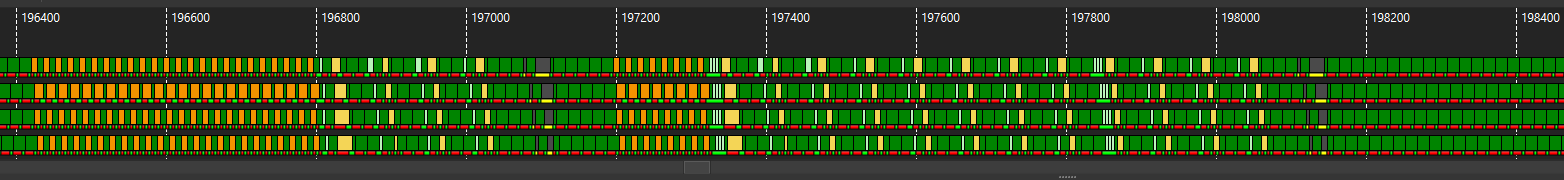
Thread trace of the v7 kernel after llirSched and the amdgcnas peephole. MFMA instructions are tightly packed across the iteration boundary, with buffer loads and LDS reads interleaved between them — the visual signature of a kernel running at 98% MFMA efficiency.

The repository includes helper scripts for this workflow. scripts/run_perf_table.py runs selected kernel versions under different scheduler configurations and reports TFLOPS, VGPRs, spills, and MFMA efficiency. scripts/process_json.py parses ATT output and computes loop timing breakdowns. The goal is to make the optimization process reproducible, not only the final kernel.

Applying the Design to BF8 and MXFP4

After the FP16 path, the repository shows how the same design transfers to lower precision formats.

BF8. The BF8 kernel keeps the same high-level structure but changes the tile shape, MFMA instruction, K width, and LDS padding. This part of the tutorial is a checklist proof: if you understand the FP16 design, the BF8 design follows from the changed instruction shape and data type. End result: 3257 TFLOPS at 99.72% MFMA efficiency on MI355 — essentially saturated.

MXFP4. The MXFP4 chapter is where the methodology earns the most. MXFP4 stores two 4-bit values per byte and uses a per-group 8-bit scale factor for every 32 elements. That single design choice — group-scaled 4-bit tensors — is the format every modern weight-quantization pipeline (W4A8, W4A16, GPTQ, AWQ-style) is converging on, and CDNA4 implements it natively on gfx950 with hardware scaled-MFMA instructions (v_mfma_scale_f32_16x16x128_f8f6f4, exposed at the Gluon level as gl.amd.cdna4.mfma_scaled).

The kernel needs an entire scale pipeline in addition to the tile pipeline. The scale pipeline is a three-step round trip:

GR → LW → LR: Global Read of scales into registers, LDS Write to convert their layout, then LDS Read to feed the scaled MFMA instruction.

The scale layout that global memory delivers is not the layout that the MFMA scaled instruction consumes, and there is no instruction that reads scales from registers into the right MFMA layout directly. So the scales make a round trip through LDS to perform a hardware-assisted layout conversion (using ds_read_tr, the transpose variant of ds_read). The tutorial schedules this extra dataflow alongside the tile pipeline so neither one stalls the MFMA, and hits 5255 TFLOPS at 92.41% MFMA efficiency end-to-end. The figure below shows how the scale pipeline interleaves with the tile pipeline.

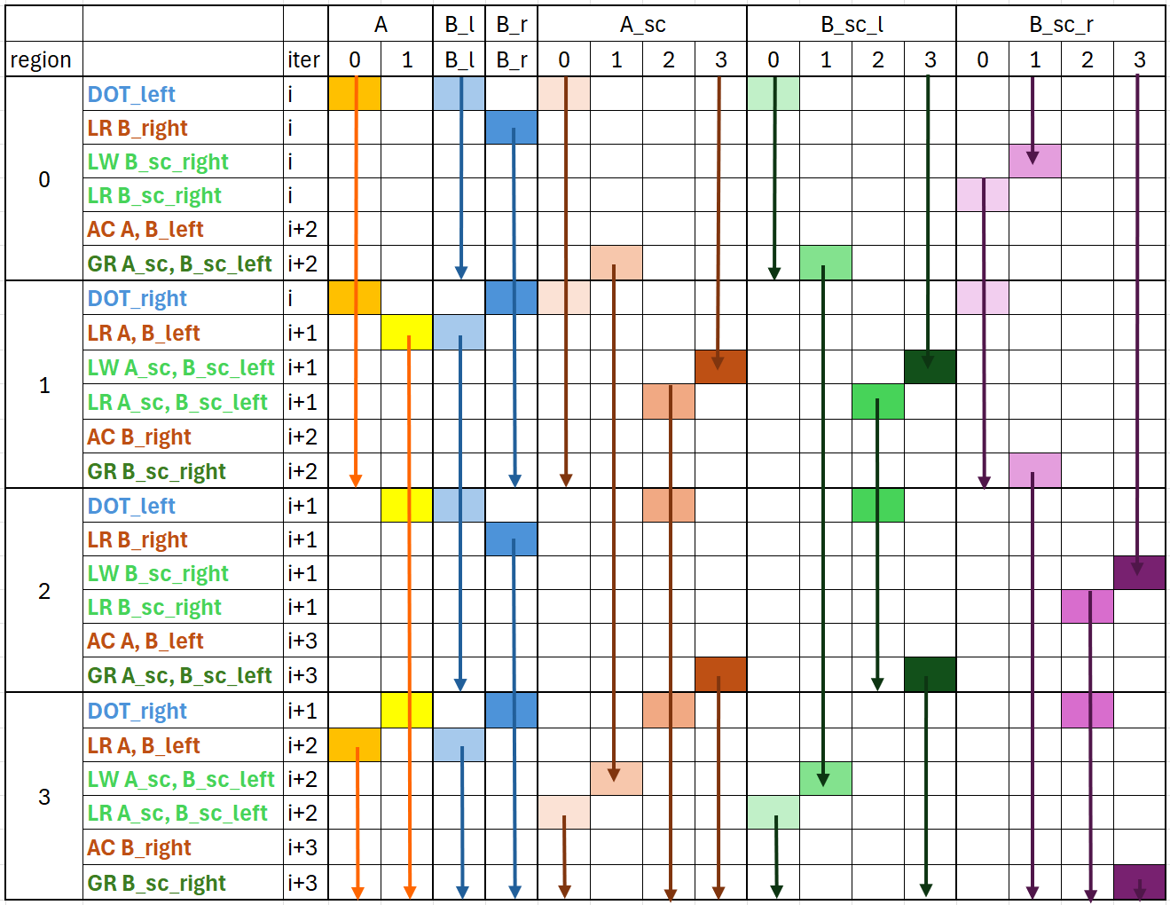
The MXFP4 tutorial adds a scale pipeline on top of the inherited tile pipeline.

What makes the MXFP4 chapter useful for an AI-inference reader is that the scale pipeline isn’t an MXFP4-only artifact. It is the general pattern for any quantized data path where the on-disk layout differs from the MFMA-consumable layout. If you are building a W4 inference kernel, an MoE expert with quantized weights, or a kernel for any future format that group-scales its tensors, you will end up with the same dataflow shape — and the tutorial’s analysis of how to schedule it without stalling MFMA is the kind of recipe that transfers.

From Kernel to Model

GEMM is the building block. To set expectations on how this work bridges to real AI workloads:

• Where the techniques apply directly. The pipeline structure, register budgeting, and LDS layout discipline transfer straight to any compute-bound kernel — fully-connected layers, expert MLPs in an MoE, the matmul half of attention, KV-cache projections. If your inference stack has a kernel sitting at 70–80% MFMA efficiency on MI350, the tutorial’s diagnostic process is the fastest way to identify what’s missing.

• What’s coming next. The same team is extending the tutorial to memory-bound GEMM, FlashAttention prefill and decode, and an MXFP4 MoE kernel — the kernels that dominate LLM inference and MoE inference today. The roadmap is public; the pace and direction are visible in the repo.

• Why this matters for evaluating MI350 for AI. The kernel source, the llirSched Triton-level pass, the amdgcnas post-assembly peephole, the run_perf_table.py reproducer, and the pinned Triton commit all ship under MIT in the same repository. The kernel that produced 99% MFMA efficiency is the same kernel you can read, run, modify, and benchmark on your own hardware — no black box, no vendor secrets.

Where to Look in docs/

The tutorial includes four standalone documents that are often more valuable than the kernel walkthrough itself:

• performance_philosophy.md — why block-level programming makes the compiler’s hard problems tractable, and how that motivates llirSched and amdgcnas.

• mfma_efficiency.md — the cycle-level metric, how to measure it, and how to read an ATT trace.

• lds_throughput.md — the bank-conflict model behind the v3 layout choice.

• memory_bandwidth_model.md — request count, request size, concurrency, and HBM bandwidth — the basis for every pipelining decision from v4 onward.

If you only have time for one read, pick the document that matches the bottleneck in your own kernel.

This post is the map. The repository is the full tutorial.

Try the Tutorial

What you’ll see: a ~3× speedup in two commands, plus a perf-table sweep that confirms the same numbers across the configurations documented in the tutorial. Setup is ~30 minutes (Triton built from source against a pinned tag); after that, two commands reproduce the journey. The peak numbers reproduce against the gfx950-tutorial-v0.1 annotated tag in triton-lang/triton, which pins a specific commit on the gfx950-tutorial branch.

The reference environment is the ROCm 7.0 PyTorch image used by the Triton CI, rocm/pytorch:rocm7.0_ubuntu22.04_py3.10_pytorch_release_2.8.0. Start a container with the GPU passthrough and ptrace permissions that rocprofv3 --att needs:

docker run -it --rm \
    --device=/dev/kfd --device=/dev/dri --group-add video \
    --cap-add=SYS_PTRACE --security-opt seccomp=unconfined \
    --shm-size=16G \
    rocm/pytorch:rocm7.0_ubuntu22.04_py3.10_pytorch_release_2.8.0

Inside the container, replace the bundled Triton with the tutorial’s pinned build:

pip uninstall -y pytorch-triton-rocm
git clone https://github.com/triton-lang/triton.git
cd triton
git checkout gfx950-tutorial-v0.1
pip install -e .
cd ..

Then clone the tutorial repository:

git clone https://github.com/ROCm/gfx950-gluon-tutorials.git
cd gfx950-gluon-tutorials

Run the naive baseline and the optimized v9 back-to-back to see the journey the tutorial walks through:

cd kernels/gemm/a16w16
# Naive baseline (~520 TFLOPS, 25% MFMA efficiency on MI355)
python bench.py --version 0 --K 8192 --dtype fp16
# Final optimized kernel (~1490 TFLOPS, 99% MFMA efficiency on MI355)
TRITON_ENABLE_LLIR_SCHED=1 TRITON_ENABLE_AMDGCN_AS=1 \
    python bench.py --version 9 --K 8192 --dtype fp16

bench.py reports do_bench (cache-warm) numbers by default. For accurate cold-cache TFLOPS that match the table and chart in this post, pass --rocprof to run_perf_table.py (shown below) — it wraps rocprofv3 --kernel-trace, runs 1000 dispatches with rotating buffers, and averages the last 100.

For a broader performance table that compares scheduler configurations across several versions, run from the repository root:

python scripts/run_perf_table.py \
  --kernel a16w16 \
  --versions 5 6 7 8 9 \
  --configs base llir llir+amdgcnas \
  --K 8192 \
  --dtype fp16 \
  --rocprof

The recommended reading order is:

1. Start with kernels/gemm/a16w16/README.md.

2. Read each version README from v0_naive through v9_beyond_hotloop (each linked from Acts I–IV above).

3. Compare the code changes with the profiler evidence.

4. Move to a8w8 for BF8 and a4w4 for MXFP4.

Dip into docs/ (see “Where to Look in docs/” above) whenever a particular bottleneck — bank conflicts, MFMA efficiency, HBM bandwidth — comes up.

Summary

In this blog you explored how a series of Gluon GEMM kernels reach near-peak matrix-engine utilization on AMD MI350/MI355 (gfx950, CDNA4) — and, just as importantly, why each step works. You walked through the FP16 path from a 520 TFLOPS naive baseline to a 1489 TFLOPS, 99% MFMA efficiency kernel, saw the v6 regression that exposes a real register-pressure problem, and followed v7–v9 as they resolve it through slicing, a post-assembly peephole pass, and XCD-aware workgroup remapping. You then saw the same design carry forward to BF8 (3257 TFLOPS, 99.72%) and MXFP4 (5255 TFLOPS, 92.41%), with the MXFP4 chapter generalizing into the scale-pipeline pattern any quantized inference kernel will eventually need.

Near-peak GEMM performance isn’t one trick. Gluon makes the sequence of design decisions explicit, the tutorial reproduces them, and the methodology transfers.

What’s next from this team. The same approach is being extended to the kernels that dominate modern AI workloads: memory-bound GEMM, FlashAttention prefill and decode, and an MXFP4 MoE kernel. The roadmap is public, the pace is visible in the repository, and future ROCm Blogs posts will dig into those kernels with the same profiler-driven methodology used here. If you are building inference kernels on MI350, follow the repo and the blog — and if you find a bottleneck the tutorial doesn’t cover yet, open an issue. The next time someone tells you AMD GPUs need vendor secrets to hit peak, you’ll know exactly where to look.

Disclaimers

The TFLOPS and MFMA-efficiency numbers in this blog were measured on a single MI355 with ROCm 7.0 and Triton built from the gfx950-tutorial-v0.1 tag. Performance varies based on hardware configuration, software versions, system topology, thermal state, and workload characteristics, and may shift as ROCm and Triton evolve. Treat the numbers as reproducible reference points for the documented setup, not as universal performance claims.

Third-party content is licensed to you directly by the third party that owns the content and is not licensed to you by AMD. ALL LINKED THIRD-PARTY CONTENT IS PROVIDED “AS IS” WITHOUT A WARRANTY OF ANY KIND. USE OF SUCH THIRD-PARTY CONTENT IS DONE AT YOUR SOLE DISCRETION AND UNDER NO CIRCUMSTANCES WILL AMD BE LIABLE TO YOU FOR ANY THIRD-PARTY CONTENT. YOU ASSUME ALL RISK AND ARE SOLELY RESPONSIBLE FOR ANY DAMAGES THAT MAY ARISE FROM YOUR USE OF THIRD-PARTY CONTENT.