A Deep Dive into LDS Optimizations on AMD Instinct MI450 GPUs

August 28, 2026 by Ognjen Plavsic, Nicola Zaghen, Lixun Zhang.

26 min read. | 6297 total words.

Software tools & optimizations

Triton, Gluon, GEMM, LDS, Performance, Optimization, Compiler, AI/ML

HPC

^{The first two authors (Plavsic, Zaghen) contributed equally to this work.}

In GEMM kernels, operands travel from global memory through the Local Data Share (LDS) into registers, where the matrix cores consume them. How efficiently data moves through the LDS is frequently the primary determinant of overall performance.

Two LDS characteristics can quietly cost a large fraction of the achievable throughput. The first arises when the in-memory layout doesn’t match the layout that the matrix cores expect for WMMA (Wave Matrix-Multiply-Accumulate), for example an N-contiguous B operand when the cores need a K-contiguous layout. A plain load from LDS cannot be vectorized in that case, but a transposed LDS load reorders the data on the fly and restores vectorized access. The second is contention on the physical LDS partitions, where warps[1] reading LDS through different ports repeatedly target the same partition and serialize their accesses. This post looks at both effects on AMD Instinct™ MI450 GPUs (gfx1250) and how to avoid them.

In this post you will learn:

• Part I – Transposed LDS loads: how the ds_load_tr cooperative-transpose instruction works and how it’s used.

• Part II – Partition conflicts: what a partition conflict is, how to structure the WMMA ctaLayout and PartitionedSharedLayout to avoid it, and how the compiler’s partition-aware allocator physically separates data across LDS partitions.

This is a deep dive aimed at Gluon and Triton kernel writers who already know the basics of authoring GEMM kernels. If you are new to Gluon kernels, start with From Naive to Near-Peak: Building High-Performance GEMM Kernels with Gluon.

A Linear Layout Refresher

Both parts of this post lean heavily on Triton’s linear layouts, so we collect the essentials here before diving in. Linear layouts were introduced in Linear Layouts: Robust Code Generation of Efficient Tensor Computation Using \(\mathbb{F}_2\); for a gentler walkthrough see Lei Zhang’s “Triton Linear Layout: Concept” and “Triton Linear Layout: Examples”.

The Basic Idea

A tensor layout is a mapping between logical tensor coordinates and the hardware resources that hold them, such as registers, lanes (the threads of a warp), warps, or shared-memory offsets. Historically each such mapping was a bespoke, hand-written attribute, and converting between any two of them needed case-by-case code – an approach whose complexity grows quadratically in the number of layouts.

A linear layout replaces those bespoke layouts with one abstraction: a map that is linear over \(\mathbb{F}_2\), the field of two elements (bits under XOR). Each input – a register, lane, or warp id – is written in binary as a bit-vector, and the layout is defined entirely by where it sends each input basis, that is, the powers of two 1, 2, 4, ... of that input. Linearity fixes everything else: the image of any index is the XOR of the images of the input bases it decomposes into. Equivalently, a linear layout is a binary matrix acting on the input bits.

Throughout this post a layout is written as a list of output offsets, one per input basis. For instance warp = [[2, 1], [1, 0]] says the input basis warp = 1 maps to [2, 1] and warp = 2 maps to [1, 0], so warp = 3 (= 1 XOR 2) maps to [2, 1] XOR [1, 0] = [3, 1].

Dividing Layouts: How an Instruction Repeats Across a Tile

A single hardware instruction, be it a wmma, a ds_load_tr or a vectorized load, has a small and fixed layout describing which lanes and registers of one instruction touch which elements of a small tile. A full operand tile is larger, so that instruction has to be repeated across it.

Linear layouts express this cleanly with left division. Left division is a block-diagonal factorization of a layout’s matrix. Recall that a linear layout is just a binary matrix over \(\mathbb{F}_2\). A matrix \(L\) is divisible on the left by \(T\) when it can be written in block-diagonal form

\[\begin{split}L = \begin{bmatrix} T & 0 \\ 0 & R \end{bmatrix}.\end{split}\]

If \(L\) is the layout of the whole tile and \(T\) is a layout factor, the quotient \(L \mathbin{/_{\ell}} T\) is the layout that remains after factoring out \(T\). When \(T\) models a complete instruction, the quotient enumerates copies of that instruction. In the ds_load_tr lowering below, however, \(T\) is only the contiguous base tile, so the quotient retains additional lane and register structure.

In Triton these repetitions show up as the reg (register) input bases of a distributed layout. That is exactly the reg dimension we manipulate later: when a warp issues several instructions, its reg bases stride across the tile, placing copy 0, copy 1, and so on.

Part I – Transposed LDS Loads

A local_load may lower to many narrow ds_load instructions when the source LDS layout and destination register layout have different contiguity. This section explains how ds_load_tr handles this mismatch using wide per-lane reads and a fixed cross-lane data exchange.

Why Is It Important?

Without ds_load_tr, a WMMA operand that has a different contiguity (say, an N-contiguous B operand) in HBM will be expensive in two ways:

• If left with a different contiguity when written to LDS, a local_load that requires it to be K-contiguous cannot use the wide ds_load_b128 vector load because the elements are strided in memory. The compiler will need to fall back to smaller loads, so each lane will issue multiple ds_load_u8/u16 instructions.

• If the shared layout has its contiguity set to K-contiguous instead so that the load vectorizes, neither TDM nor async_copy can perform this reordering while copying from HBM to LDS. The operand must first be loaded into registers and then stored to LDS, shifting the overhead of changing contiguity to the store side. The compiler will need to fall back to smaller stores, so each lane will issue multiple ds_store_b8/b16 instructions in a strided K-contiguous pattern.

Using ds_load_tr avoids both tradeoffs. Every lane can issue vectorized LDS reads (64 or 128 bits depending on the data type), then the hardware redistributes the data across the lane groups so that the loaded data matches the destination layout. This gives a gain in terms of both instruction count and register pressure. A large number of small ds_load instructions clustered together can also exhaust the DSCNT counter, forcing the hardware to wait before the local_load completes.

For a concrete example, consider the fp16 forward attention kernel from Triton’s 06-fused-attention.py, compiled for gfx1250 without causal masking using BLOCK_M = 128, BLOCK_N = 128, HEAD_DIM = 256, and eight warps. With transposed loads enabled, the generated assembly contains 128 ds_load_tr16_b128 instructions. Disabling transposed loads replaces them with 1024 ds_load_u16 instructions, increases VGPR usage from 308 to 512, and causes 233 VGPRs to spill.

What Does ds_load_tr Do?

MI450 provides several ds_load_tr variants. We focus on ds_load_tr8_b64 and ds_load_tr16_b128 as representative examples because they appear most often in practice; both perform a cooperative transposed load across a full 32-lane warp as 4 independent groups of 8 lanes. The b64/b128 suffix gives the number of bits read per lane, while tr8/tr16 gives the element width. Figures 1a and 1b give the per-lane ownership of a 32x8 tensor before and after the redistribution for the two variants.

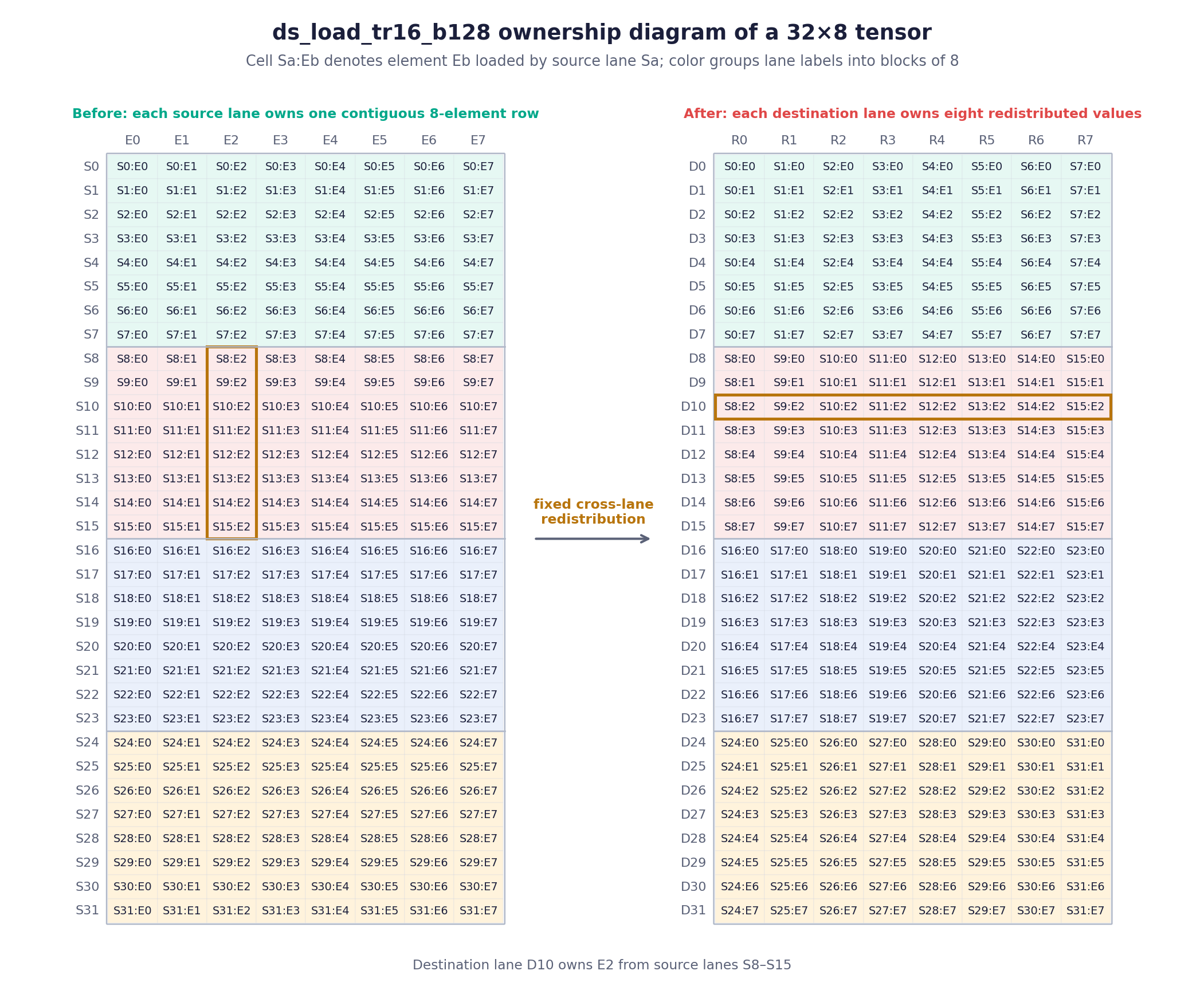
Figure 1a: Ownership diagram of a 32x8 tensor for ds_load_tr16_b128. The left side shows the eight elements read by every source lane S; the right side shows the eight values held by every destination lane D after four independent 8x8 transposes.

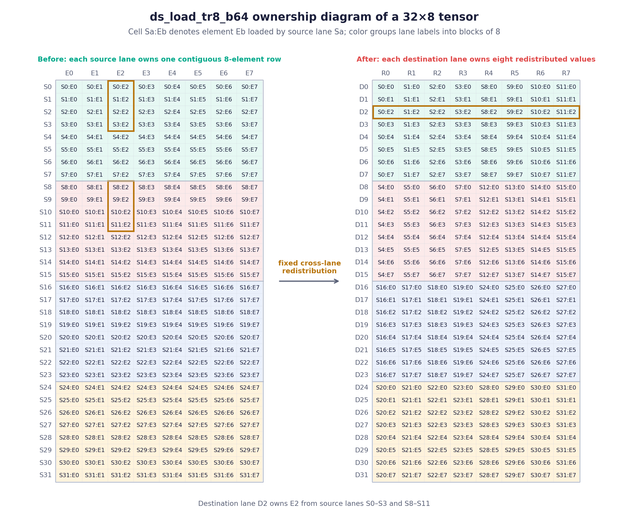
Figure 1b: Ownership diagram of a 32x8 tensor for ds_load_tr8_b64. Unlike the contiguous groups used by ds_load_tr16_b128, each source group combines two runs of four lanes. In each map, color groups its S or D lane labels into blocks of eight.

The data loaded by this instruction is transposed in tiles of size N x T, where N = 8 is the number of contiguous elements read by each lane and T = 8 is the number of lanes in a group. For both ds_load_tr16_b128 and ds_load_tr8_b64, this forms an 8x8 tile of 8/16-bit elements that the hardware transposes so destination lane D_i receives column E_i.

For example, within one 8-lane group (S0…S7 refer to source lanes 0…7):

• Destination lane D0 receives column E0: [S0:E0, S1:E0, S2:E0, S3:E0, S4:E0, S5:E0, S6:E0, S7:E0], the first b16 element loaded by each source lane.

• Destination lane D1 receives column E1: [S0:E1, S1:E1, S2:E1, S3:E1, S4:E1, S5:E1, S6:E1, S7:E1], the second b16 element loaded by each source lane.

• Destination lane D8 receives column E0 of the next independent group: [S8:E0, S9:E0, S10:E0, S11:E0, S12:E0, S13:E0, S14:E0, S15:E0]. Because N equals the group size, every lane in a group draws from all 8 lanes of that group.

The ds_load_tr8_b64 variant uses a different lane distribution than the b16 version: each source group combines two runs of 4 lanes. For example, destination lanes D0 through D7 draw from source lanes S0 through S3 and S8 through S11. Figures 2a and 2b assemble these per-group 8x8 tiles into the full 16-bit and 8-bit WMMA B-operand tiles.

Figure 2a: gfx1250 lane ownership for a complete 16-bit WMMA B-operand tile. Each 16x16 panel corresponds to one ds_load_tr16_b128 instruction.

Figure 2b: gfx1250 lane ownership for a complete 8-bit WMMA B-operand tile. Each 16x16 panel corresponds to one ds_load_tr8_b64 instruction, with each source group split into two runs of four lanes.

The example above shows how the instruction behaves when the per-lane LDS addresses form an 8x8 slice of a WMMA operand. This is not a hardware restriction: each lane can read from an independent LDS address as long as its own 64/128-bit read is contiguous, and the hardware applies the same fixed redistribution regardless of the addresses or what the bits represent.

Because the redistribution does not depend on the relationship between the addresses, “transpose” is only the mental model for one particular address pattern; the instruction can support more general data movement. Eligibility depends only on whether the requested (register, lane) -> offset mapping fits the instruction’s fixed data-movement pattern. Representing both as linear layouts lets the compiler test that match directly instead of detecting a high-level transpose operation. Figure 3 illustrates this flexibility: each lane supplies an independent LDS address, and ds_load_tr applies the same fixed cross-lane redistribution to whatever vectors those addresses select.

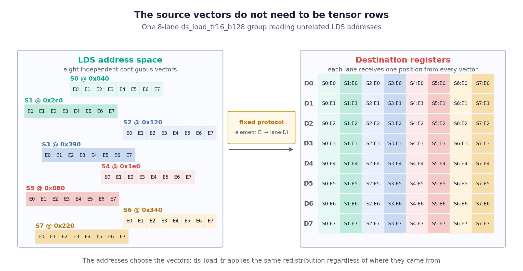
Figure 3: ds_load_tr does not require the source addresses to describe rows of a geometric tile. Each lane supplies an independent LDS address, while the instruction applies the same fixed cross-lane redistribution to the selected vectors.

From the perspective of LDS bank conflicts, ds_load_tr behaves like a regular ds_load. The hardware selects banks from the LDS addresses issued by the lanes; the cross-lane redistribution happens afterward. Bank conflicts should therefore be analyzed using the source LDS layout, not the destination register layout.

Lowering local_load to ds_load_tr in Triton

Triton implements this lowering in MemoryOpToLLVM.cpp as part of the conversion from TTGIR to LLVM IR. The lowering converts the shared and destination encodings into linear layouts, then computes cvt = dstLL.invertAndCompose(sharedLL), which maps each destination hardware position (register, lane, warp) to its source LDS offset.

Consider a toy tensor<32x8xbf16> example with a single warp, M = 32, K = 8, and 8 elements per lane:

#shared = #ttg.swizzled_shared<{vec = 1, perPhase = 1, maxPhase = 1, order = [0, 1]}>
#dst    = #ttg.linear<{register = [[0, 1], [0, 2], [0, 4]],
                       lane     = [[1, 0], [2, 0], [4, 0], [8, 0], [16, 0]],
                       warp = [], block = []}>

We have that #shared’s order = [0, 1] makes dim 0 (M) the LDS-contiguous dimension, while #dst is already expressed as a linear layout (this is the “Identity” case a few paragraphs down). Composing them:

     dstLL                          sharedLL                       cvt = dstLL.invertAndCompose(sharedLL)
     (register,lane) -> [M,K]       offset -> [M,K]                (register,lane) -> [offset]
     -------------------------      -----------------              --------------------------------
     register=1  -> [ 0, 1]            1 -> [ 1, 0]                register=1  -> [ 32]
     register=2  -> [ 0, 2]            2 -> [ 2, 0]                register=2  -> [ 64]
     register=4  -> [ 0, 4]            4 -> [ 4, 0]                register=4  -> [128]
     lane=1      -> [ 1, 0]            8 -> [ 8, 0]                lane=1      -> [  1]
     lane=2      -> [ 2, 0]           16 -> [16, 0]                lane=2      -> [  2]
     lane=4      -> [ 4, 0]           32 -> [ 0, 1]                lane=4      -> [  4]
     lane=8      -> [ 8, 0]           64 -> [ 0, 2]                lane=8      -> [  8]
     lane=16     -> [16, 0]          128 -> [ 0, 4]                lane=16     -> [ 16]

invertAndCompose builds cvt by taking each dstLL target [M,K] and matching it to each target of sharedLL, then reading that basis’s offset – e.g. dstLL has register=4 -> [0,4] which matches sharedLL’s 128 -> [0,4], so cvt will have register=4 -> [128]. sharedLL has to be surjective onto [M,K] for this lookup to always succeed.

The instruction is modeled in terms of the smallest layout factor it operates on, so we can avoid writing bespoke code that pattern-matches specific shapes like “this destination layout looks like a transpose of shared memory”. This is because an instruction is defined by how it moves data on the hardware and not by a map from (register, lane, warp, block) to tensor coordinates. A tile is the contiguous factor required by the instruction, and a destination layout cvt can use that instruction only if divideLeft(cvt, tile) has a result. The quotient describes the remaining structure after tile is factored out; fullTile supplies the remaining lane and register mapping for one complete instruction.

The lowering models ds_load_tr16_b128 with two related layouts:

• tile = identity1D(8, lane, offset) describes the contiguous part required for instruction selection. For a fixed destination register, destination lanes 0 through 7 request 8 consecutive LDS offsets.

• fullTile extends tile across all the lanes and registers that participate in one instruction. Its offset dimension identifies an element within the contiguous base tile, while its addr dimension identifies which lane’s LDS read supplies that element. The order in which the remaining lane and register bases are assigned to addr encodes the instruction’s data exchange pattern. The two instructions use the same base tile but distribute it differently across the full instruction. Figures 4a and 4b sample one ownership panel of each variant, showing how those bases map from (lane, register) to (offset, addr).

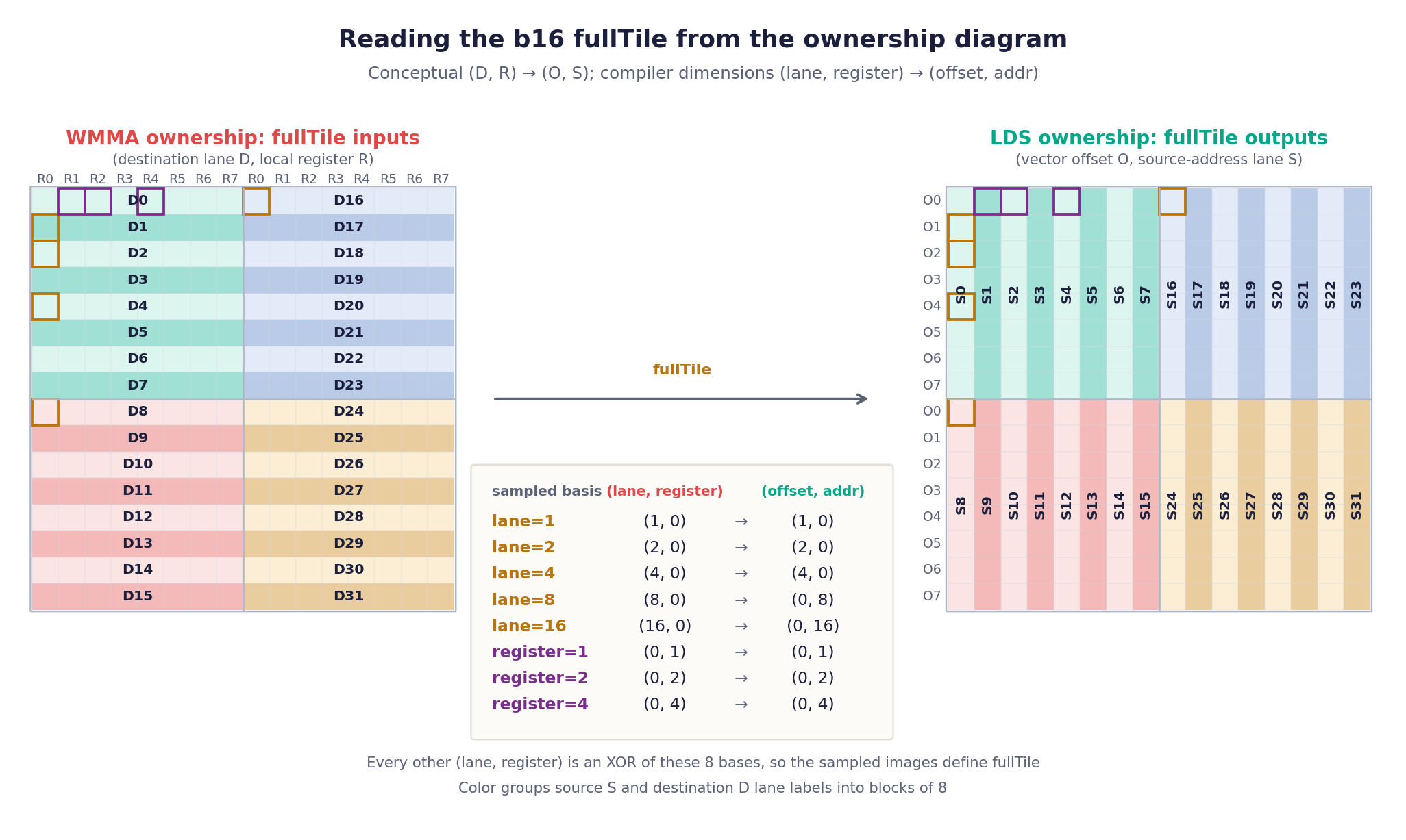
Figure 4a: Reading the b16 fullTile from one ds_load_tr16_b128 ownership panel in Figure 2a. Each logical element pairs a destination (D, R) with its source (O, S), corresponding to the compiler dimensions (lane, register) and (offset, addr). Sampling the five lane bases and three register bases is enough to define the layout, because every other position is an XOR of those bases.

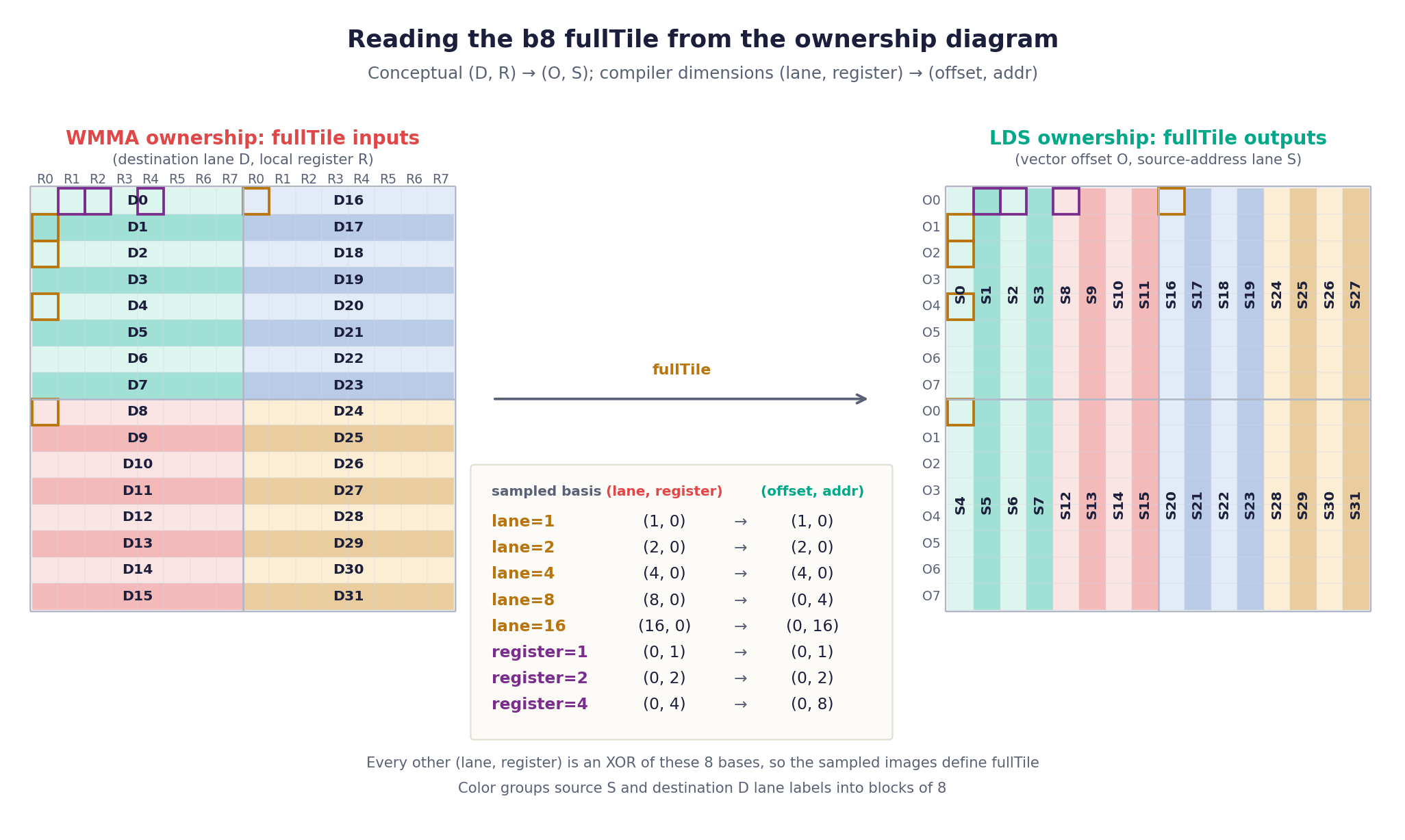
Figure 4b: The same sampling for one ds_load_tr8_b64 ownership panel in Figure 2b. The lane and register bases are assigned to addr in a different order, so only two of the eight images change: lane=8 now selects source lane S4 instead of S8, and register=4 selects source lane S8 instead of S4. That is what splits each group into two runs of four source lanes, visible in the source panel as the color changing halfway across each eight-register region.

The two main lowering steps that follow are:

• Eligibility check: Build the access mapping from destination hardware positions to LDS offsets, then check whether it contains the data movement pattern required by the instruction.

• Instruction emission: Factor that pattern out of the access mapping, derive the LDS address read by each runtime lane and warp, and emit one instruction for each remaining repetition.

These are operations on layout mappings rather than on linear layouts specifically. Triton represents those mappings with linear layouts and performs the operations using composition, inversion, and division. Figure 5 visualizes the eligibility check on the cvt basis mappings, while Figure 6 follows the sequence of mappings used to derive the runtime LDS addresses.

The compiler first checks divideLeft(cvt, tile). The cvt layout must be divisible by tile in order for the lowering to work. The figure below applies this check to a minimal one-warp tensor<32x8xbf16> example. It mirrors the valid, scrambled-valid, and invalid cases in Triton’s ds_transpose_ll regression tests in test/Conversion/amd/ds_transpose_gfx1250.mlir.

Figure 5: ds_load_tr16_b128 eligibility constrains the first 3 lane bases of cvt – the (register, lane) -> [offset] map obtained by composing the destination layout with the inverse of the shared layout. Those bases must match the base tile (lane=1,2,4 -> [1],[2],[4]), while every remaining basis must map to a multiple of 8. The repetition bases can be rearranged (middle); swapping two of the required lane bases (right) leaves divideLeft with no result and the load falls back to scalar.

If divideLeft succeeds, its quotient describes how repetitions of tile are laid out in cvt, but in a reduced coordinate space where the tile itself has been factored out. The lowering computes reps = zerosLike(tile) * quotient to lift it back into cvt’s full offset space. This restores the tile’s lane bases as zero, so reps maps each destination register/lane/warp position to the base LDS offset of its tile rather than to a position within that tile.

The lowering then computes addrToOffset = fullTile.invert().compose(reps). fullTile.invert() maps a position within one instruction, (offset, addr), to the destination register and lane that receive it; composing with reps maps that destination position to its LDS tile base. Here addr enumerates the independent source reads issued by the lanes of one instruction. The compiler therefore renames the addr bases of addrToOffset to the lane bases of addrLayout and adds the warp bases from reps. Evaluating addrLayout with the runtime lane and warp IDs gives the LDS address that each lane must read.

Figure 6: The layout pipeline used after divideLeft succeeds. The quotient removes the base tile, reps lifts its placement back into the original offset space, and fullTile.invert() translates the instruction’s (offset, addr) coordinates through reps. The final addrLayout maps runtime lane and warp IDs directly to the LDS address issued by each lane.

Key Takeaways

• Transposed LDS loads remove the cost of a contiguity mismatch. When a WMMA operand sits in LDS with a contiguity that differs from what the register layout needs, an ordinary local_load degrades into many narrow ds_load instructions. ds_load_tr instead lets every lane issue one wide read and has the hardware redistribute the data into the destination layout, cutting instruction count and register pressure.

• ds_load_tr eligibility is a layout-matching problem, not transpose detection. Because the instruction applies a fixed cross-lane pattern, the compiler expresses both layouts as linear layouts and uses left division (divideLeft) to test whether the required (register, lane) -> offset map factors into the instruction’s fixed tile. If it does, the load is eligible.

Part II – Partition Conflicts

Transposed loads optimize a single warp’s read out of LDS. Partition conflicts are about what happens when multiple warps read LDS at the same time. Each Workgroup Processor (WGP)[2] on MI450 contains four SIMD (vector) units, organized into two physical pairs. Pair A holds SIMD 0 and SIMD 2; Pair B holds SIMD 1 and SIMD 3. Warps are dispatched round-robin – warp N runs on SIMD N mod 4 – so even-numbered warps always land on Pair A and odd-numbered warps on Pair B.

The WGP also holds six 64 KiB hardware memory partitions. The split is fixed in hardware: five belong to LDS, giving its 320 KiB capacity, and the sixth backs the L0 vector cache. These partitions are the unit of contention for the rest of this post.

Each SIMD pair sends its LDS request to a shared LDS/L0 arbiter, which owns two ports, L and C, each running at 256 B/cycle and each able to reach every partition. When the arbiter can grant the two incoming requests separate ports, they access LDS in the same cycle for a combined 512 B/cycle; otherwise they serialize and effective bandwidth halves to 256 B/cycle. Figure 7 shows this datapath: both SIMD pairs feed the shared arbiter, whose two ports reach all six hardware partitions.

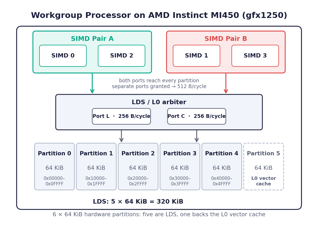
Figure 7: The LDS datapath of a single MI450 Workgroup Processor: both SIMD pairs feed a shared LDS/L0 arbiter whose two ports reach all six hardware partitions.

The Partition-Conflict Rule

A partition conflict occurs when warps from different SIMD pairs issue LDS accesses to the same physical LDS partition in the same cycle.

Two conditions must hold at once:

• Location – both accesses target the same partition.

• Time – both are issued in the same cycle.

Only cross-pair accesses can satisfy both conditions, since a pair presents at most one LDS request to the arbiter per cycle. When two such accesses do coincide in partition and cycle, the arbiter serializes them and LDS bandwidth halves. Breaking either condition therefore avoids the conflict. Triton and Gluon have no control over the cycle on which a warp issues its access, so location is the condition we can act on.

Separating locations is what the rest of this part builds, step by step:

• Why the standard WMMA layout conflicts on operand A.

• How writing the CTA layout as a linear layout lets us swizzle the two pairs apart.

• Why that swizzle is not enough on its own, and what a PartitionedSharedLayout adds.

• How the choice of ctaLayout also sets the TDM cost of storing the operands in LDS.

• How the partition-aware allocator makes the separation physical.

• How the resulting local loads are lowered with almost no run-time cost.

• How much the separation actually buys, measured with a kernel that does nothing but read LDS.

Note

Because time is one of the conditions, a partition conflict is not a deterministic quantity the way a bank conflict is. Threads within a warp run in lockstep, so bank conflicts are countable. Separate warps, however, drift relative to one another, so we model the four warps as if they issued the same instruction on the same cycle. Under that assumption separating locations removes the conflict outright; in practice it drives its probability down rather than strictly to zero.

Why the Standard WMMA Layout Conflicts

Consider a 4-warp GEMM with the standard WMMA CTA layout, initially represented in Gluon by warpsPerCTA = [2, 2]. warpsPerCTA is a bespoke shorthand for how warps are laid out across the output tile – the same mapping Gluon now also expresses generically as the WMMA ctaLayout, which we come to shortly. It arranges the four warps in a 2x2 grid over the tile, as shown in Figure 8:

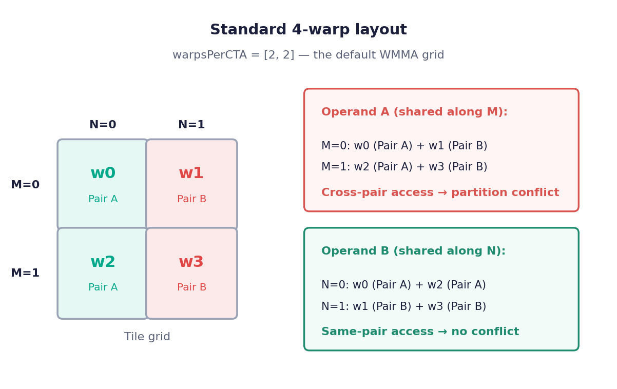
Figure 8: With the default warpsPerCTA = [2, 2] layout, each M-row is shared by one Pair A warp and one Pair B warp.

Each warp at tile (m, n) reads the A rows for its M-position and the B columns for its N-position. An “M-row” here is not a single matrix row, but the band of M rows one warp covers with a single WMMA instruction. Warps in the same M-row read the same A data. In this layout, w0 (Pair A) and w1 (Pair B) share M-row 0, and w2 (Pair A) and w3 (Pair B) share M-row 1.

Since both pairs read the same bytes, those bytes live in one partition, and identical data cannot be spread across partitions. This layout therefore locks in the location condition on A: the two pairs are guaranteed to be co-located, and only their relative timing decides whether a given access pair actually collides. That is exactly the situation to avoid, since it leaves nothing under our control. Operand B is fine here: the warps sharing an N-column (w0+w2, w1+w3) belong to the same pair.

CTA Layout as a Linear Layout

Recall from the linear layout refresher that a layout maps hardware inputs to tensor coordinates by assigning each input basis an [M, N] offset and composing them with XOR. The ctaLayout is the slice of this description that places warps over the output tile: its warp bases assign each warp its tile, and its reg bases enumerate the repetitions when a single warp covers several tiles.

The bespoke warpsPerCTA = [2, 2] becomes the following ctaLayout:

ctaLayout = {
    warp = [[0, 1], [1, 0]],
}

We specify only the warp bases: they already cover the output tile (the layout is surjective), so Triton fills in the reg repetitions automatically later in the pipeline. Reading it, warp = 1 maps to [0, 1] and warp = 2 to [1, 0], so w3 (which decomposes into warp = 1 XOR warp = 2) lands on [0, 1] XOR [1, 0] = [1, 1].

The swizzled layout keeps the same four warps but changes warp = 1 to move along M:

ctaLayout = {
    reg  = [[2, 0]],
    warp = [[2, 1], [1, 0]],
}

warp = 1 now maps to [2, 1] instead of [0, 1]. With this change the warp bases alone no longer cover the tile, so we add an explicit reg = [[2, 0]] basis to restore surjectivity. That reg basis is the repetition: w1 on its second iteration combines warp = 1 and reg = 1, landing on [2, 1] XOR [2, 0] = [0, 1].

The two ctaLayouts above differ in exactly one place: the input basis warp = 1, which determines whether warps from different pairs read the same M-rows. In the standard layout it maps to [0, 1] – a pure N move – which is precisely why cross-pair warps landed on the same M-row and read the same A bytes. The swizzle changes it to [2, 1], whose nonzero M component pushes those cross-pair warps onto different M-rows, so they read different A data. Figure 9 shows the resulting layout, with the two pairs on disjoint M-rows.

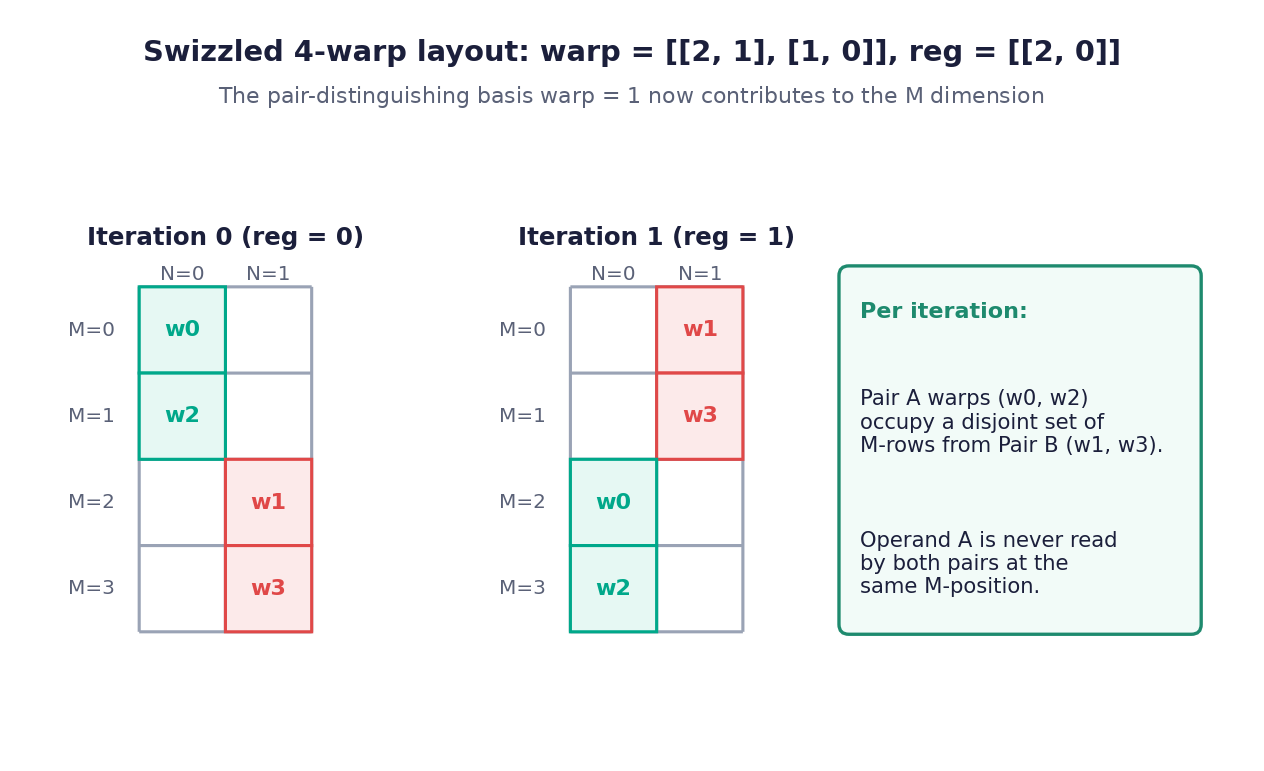
Figure 9: With the swizzled layout, all Pair A warps occupy one set of M-rows and all Pair B warps a disjoint set. The cross-pair sharing on A is gone.

When the ctaLayout Is Not Enough: PartitionedSharedLayout

Swizzling the ctaLayout guarantees that cross-pair warps address different tiles. But it says nothing about which physical partition those tiles land in. If the entire operand fits inside a single 64 KiB partition – for example A [128, 128] in fp16 is exactly 32 KiB – then every warp reads from that one partition regardless of its tile, and Pair A and Pair B collide again.

PartitionedSharedLayout is the Gluon mechanism that does this splitting. It takes four parameters – num_partitions, num_groups, partition_dim, and partition_layout – which together serve two purposes. First, they tell the allocator which logical pieces must live in separate physical partitions, so it can place them in different 64 KiB regions. Second, they give the compiler enough information to build a unique mapping between shared-memory addresses and logical tensor coordinates, which is what lets it lower every load and store to the right address.

The parameters are easiest to understand by deriving them from a concrete kernel. Consider the following GEMM: C[128, 128] = A[128, K] * B[K, 128], four warps, fp16, using the swizzled ctaLayout from the previous section. That layout’s tile is 64x32 – a 4x2 block of 16x16 warp tiles – and it repeats across the 128x128 output.

Figure 10 draws the whole picture, and every parameter can be read straight off it. In the center is the C[128, 128] output as an 8x8 grid of 16x16 warp tiles. The swizzled ctaLayout tile is the 64x32 block outlined by the dividers (a 4x2 group of warp tiles); it repeats 2 x 4 = 8 times to cover C. Down the left edge is operand A sliced along M; along the top is operand B sliced along N. Each such slice is a piece – a contiguous band of the operand along the slice dimension – and the figure labels them pc0, pc1, and so on.

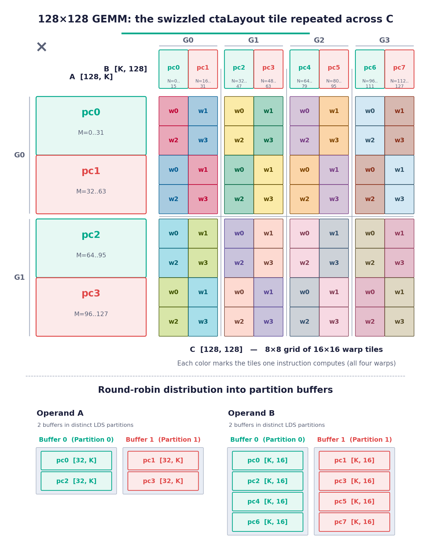
Figure 10: The swizzled ctaLayout tile repeated across C, where each color marks the tiles one instruction computes across all four warps. A is sliced along M into 2 x 2 = 4 pieces (groups G0-G1); B along N into 2 x 4 = 8 pieces (groups G0-G3). The lower panels show the round-robin distribution: even pieces to Partition 0, odd pieces to Partition 1.

partition_dim is the axis we slice along. The swizzled ctaLayout already spreads the two SIMD pairs along the non-K dimension, so that is where we cut: partition_dim = 0 (M) for A, partition_dim = 1 (N) for B.

num_partitions follows from the conflict rule. The swizzle splits the warps by pair – w0, w2 are Pair A; w1, w3 are Pair B – and in every instruction each pair reads a different band of partition_dim. Give each pair its own buffer (Pair A -> partition 0, Pair B -> partition 1) and the conflict is gone: two pairs -> num_partitions = 2. Note this logical count is not the five physical partitions of the WGP: the conflict is strictly between the two SIMD pairs, so two buffers in two distinct physical partitions are all that is needed; the five physical partitions simply give the allocator room to place those two buffers apart.

num_groups exists because the data for each partition can be interleaved along partition_dim: walking down operand A the pieces alternate pc0 -> P0, pc1 -> P1, pc2 -> P0, pc3 -> P1. One full (P0, P1) cycle is a group, and num_groups counts how many times it repeats – the G brackets in the figure. Equivalently, it is how many times the ctaLayout tile repeats along partition_dim: A 128 / 64 = 2; B 128 / 32 = 4.

partition_layout is the last parameter: it describes how a single piece is laid out within its partition. This is an ordinary PaddedSharedLayout, whose order and padding are chosen to keep the intra-piece accesses free of bank conflicts. Putting it together, the two operands are:

from triton.experimental.gluon.language.amd.gfx1250 import PartitionedSharedLayout

a_shared = PartitionedSharedLayout(
    num_partitions=2,
    num_groups=2,
    partition_dim=0,             # slice A along M
    partition_layout=a_inner_layout,
)

b_shared = PartitionedSharedLayout(
    num_partitions=2,
    num_groups=4,
    partition_dim=1,             # slice B along N
    partition_layout=b_inner_layout,
)

Choosing the ctaLayout to Reduce TDM Traffic

The number of pieces is not just bookkeeping – it determines how the operand is loaded from global memory. On MI450 the Tensor Data Movement engine (TDM) copies a tensor into LDS, and each TDM instruction moves at most one piece per warp – a hardware constraint tied to the striding patterns a warp can write. The instruction count therefore follows directly from the piece count:

\[\text{TDM instructions} = \left\lceil \frac{\text{number of pieces}}{\text{number of warps}} \right\rceil\]

With four warps:

• Operand A: 4 pieces, 4 warps -> a single TDM instruction covers all pieces.

• Operand B: 8 pieces, 4 warps -> two TDM instructions are needed.

The piece count – and therefore the TDM cost – is a consequence of the WMMA ctaLayout you pick. The layout above assigns each warp a single 16x16 tile, which makes the pieces small: operand B ends up as eight [K, 16] strips. If instead we choose a coarser ctaLayout where each warp covers a four-tile strip of partition_dim, the pieces grow and their count drops. Figure 11 shows this alternative: warps = {[2, 4], [1, 0]} gives a 64x128 tile that tiles C in 2x1 blocks (stacked along M).

Figure 11: Making each warp span a four-tile strip yields bigger, fewer pieces. Colors again mark the tiles computed by each instruction. Operand A is unchanged (four [32, K] pieces, num_partitions = 2), but operand B collapses from eight [K, 16] pieces to two [K, 64] pieces (num_groups = 1).

Two things fall out of this choice. First, TDM cost drops: with four warps, operand B’s two pieces now fit in a single TDM instruction instead of two. Second, the larger pieces use the memory system better – B is N-contiguous, and in fp16 a 128-byte cacheline holds 64 N-elements, so a [K, 64] piece is exactly one cacheline while the old [K, 16] piece filled only a quarter of one. The separation between the pairs is untouched; we have only traded piece granularity for fewer, better-utilized transfers, so the WMMA ctaLayout and the PartitionedSharedLayout parameters must be chosen together.

Reading the new parameters off the coarser tile, operand A is unchanged, but operand B now has a single group (its two pieces are one (P0, P1) cycle):

a_shared = PartitionedSharedLayout(
    num_partitions=2,
    num_groups=2,
    partition_dim=0,             # slice A along M
    partition_layout=a_inner_layout,
)

b_shared = PartitionedSharedLayout(
    num_partitions=2,
    num_groups=1,                # was 4: B is now two [K, 64] pieces
    partition_dim=1,             # slice B along N
    partition_layout=b_inner_layout,
)

How the Partition Guarantee Is Enforced: Partition-Aware Allocation

The linear layout says which partition a piece belongs to; the allocator is what makes those partitions land in different physical 64 KiB regions of LDS. Triton’s shared-memory allocator is a greedy interval-placement algorithm from the classic paper “Algorithms for Compile-Time Memory Optimization”, and the partitioned case is a small extension of it (Allocation.cpp).

The base algorithm treats each buffer as a rectangle in (time x offset) space – its liveness range along time and its size along offset – and greedily places each buffer at the lowest offset that does not overlap any other buffer live at the same time. The extension for partitioned tensors adds two ingredients.

First, when a local_alloc uses a PartitionedSharedEncoding, the allocator creates num_partitions buffers (each holding all of that partition’s groups concatenated, so its size is pieceSize x num_groups) and marks them all as mutual neighbors. Neighbors are required to occupy different physical partitions.

Second, placement is made partition-aware in two stages:

• Stage 1 (initial placement). In the base algorithm this step scans the open free slots from the lowest offset up and, at each slot, picks the first candidate whose liveness fits, gives it that offset, and splits the leftover space into new slots.

  Partition awareness adds one gate to that choice: a candidate is only accepted if it lands in a different physical partition than its already-placed neighbors. This can leave the current slot blocked – every candidate that fits here would collide with a neighbor’s partition. When that happens the allocator reopens the slot at a higher offset, past the neighbors’ partitions, so a candidate becomes acceptable there. Because the offset only ever moves up, the algorithm keeps making progress. Figure 12 traces four iterations of this stage-1 placement, growing the search height until each partition buffer finds a partition free of its neighbors.

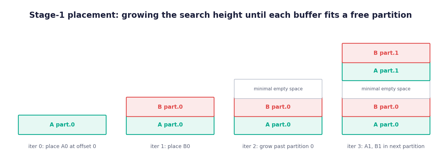
Figure 12: Stage-1 placement grows the search height until each partition buffer finds a partition free of its already-placed neighbors.

• Stage 2 (interference refinement). In the base algorithm the initial offsets can still leave some buffers overlapping, so this step builds an interference graph – an edge between any two buffers that are live at the same time and whose byte ranges overlap – colors it, and pushes each buffer above the ones it interferes with, repeating until nothing overlaps.

  Partitions need this step too, because the offset bumping this stage performs can itself slide a buffer into the same physical partition as one of its neighbors, undoing what stage 1 established. So partition awareness adds one more kind of interference edge: two neighbors that share a physical partition. When that edge is resolved, the buffer is bumped past the neighbor’s partition rather than just past its bytes, restoring the guarantee.

How Partitioned Local Loads Are Lowered

The ctaLayout and the allocator settle everything at compile time; the last question is what the load itself has to compute at run time. Each operand carries a distributed layout, mapping a thread’s (register, lane, warp) to tensor coordinates, and a shared layout, mapping an LDS location to the same coordinates. The backend emits their composition, cvt: (register, lane, warp) -> offset. A partitioned shared layout simply adds a second output dimension, so the conversion yields an (offset, partition) pair – which physical buffer to read from, alongside where in it. Figure 13 shows this composition for a 64x64 partitioned operand A, highlighting the bases that feed the new partition coordinate.

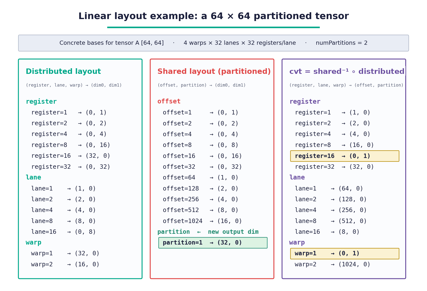
Figure 13: A partitioned shared layout adds a partition output dimension. Composing it with the distributed layout yields cvt: (register, lane, warp) -> (offset, partition); the highlighted bases are the ones that feed the new partition coordinate.

Like every linear-layout output, the partition index is an XOR of basis contributions, and each one resolves cheaply: the register term is a compile-time constant, the warp term is a runtime value but loop-invariant, and lane usually does not feed partition at all. Base-pointer selection therefore lifts out of the loop entirely. The backend resolves the warp-dependent part once and pre-computes a small array of reordered base pointers, one per partition, which each load indexes with a constant that folds to a literal.

This mirrors what the backend already does without partitioning, where a single dynamic address computation is hoisted ahead of the loop and the body left fully static. Partitioning only adds the base-pointer array alongside it, so the run-time price is a one-time setup proportional to the number of partitions rather than to the number of loads, and the address math inside the K loop stays the same pure-XOR expression as the baseline.

Measuring It: An LDS Bandwidth Microbenchmark

Everything above is a compile-time construction. To measure what it buys, we isolate the effect in a microbenchmark that changes only the shared layout – same shape, same instruction count, same vector width, same bank behavior.

What is loaded. The kernel reads a [NUM_WARPS, N] fp16 tensor out of LDS and does nothing else. Scaled down to [4, 256] so that the bases fit on the page, its layouts are:

distributed (blocked)           shared, plain              shared, partitioned
(reg, lane, warp) -> (d0, d1)   offset -> (d0, d1)         (offset, partition) -> (d0, d1)

reg  =  1 -> (0,   1)           offset =   1 -> (0,   1)   offset =   1 -> (0,   1)
reg  =  2 -> (0,   2)           offset =   2 -> (0,   2)   offset =   2 -> (0,   2)
reg  =  4 -> (0,   4)           ...                        ...
lane =  1 -> (0,   8)           offset = 128 -> (0, 128)   offset = 128 -> (0, 128)
lane =  2 -> (0,  16)           offset = 256 -> (1,   0)   offset = 256 -> (2,   0)
lane =  4 -> (0,  32)           offset = 512 -> (2,   0)   partition = 1 -> (1,   0)
lane =  8 -> (0,  64)
lane = 16 -> (0, 128)
warp =  1 -> (1,   0)
warp =  2 -> (2,   0)

Four properties of the kernel follow directly from those bases:

• One row per warp. The warp bases of the distributed layout carry dim 0 and nothing else, so warp w owns row w in its entirety and touches no other row.

• One 512-byte window per load. The register and lane bases cover dim 1 contiguously at 8 fp16 apiece, which is 128 bits per lane, so a warp spans 512 bytes with a single ds_load_b128. The measured runs use a much longer row, which only adds register bases striding along dim 1, and with them the back-to-back loads that are timed.

• No bank conflicts either way. That same contiguity means the lanes read consecutive 16-byte chunks, and ds_load_b128 services the warp in groups of 16 lanes, so each group covers all 64 banks exactly once.

• The two shared layouts differ in one place only: which partition a row ends up in. In the plain layout the four rows sit in one contiguous buffer, so they all share a single partition. In the partitioned layout the rows alternate between two. Warp w owns row w, so this is what puts it on partition w % 2.

The tensor is sized so the unpartitioned baseline fits inside a single 64 KiB partition, which is the regime where it is guaranteed there is a conflict to resolve. The compiled LDS size is the evidence that the placement actually happened. For a 64 KiB tensor the baseline allocates one 64 KiB buffer at offset 0, while the partitioned version allocates two 32 KiB buffers and is forced to push the second to the 64 KiB boundary, for 96 KiB total.

How bandwidth is computed. Each warp issues a run of back-to-back ds_load_b128, bracketed by two reads of s_get_shader_cycles_u64, the shader-clock cycle counter. A barrier before the opening clock read lines the warps up so their runs overlap, and a second barrier after the last load makes sure every load has retired before the closing clock read. The warps together read the tensor exactly once, so bandwidth is its size in bytes divided by the recorded cycles.

Steady-state bandwidth. That number divides by everything the clock counted, including a fixed startup and drain cost – the two clock reads and the barrier, plus one un-overlapped LDS round trip for the first access. That cost does not grow with the burst, so it understates bandwidth, and understates it worse the faster the kernel streams, since a fixed cost is a larger share of a shorter run. Modeling a burst as

\[\text{cycles} = \text{fixed} + \frac{\text{bytes}}{\text{rate}}\]

and fitting cycles against bytes over a range of burst lengths recovers the rate as the reciprocal slope, with the fixed cost falling out as the intercept.

Results. At four warps over a 64 KiB working set, 32 loads per warp:

layout	measured cycles	LDS	raw B/cycle	steady B/cycle	peak B/cycle
plain	323	64 KiB	202.9	255.4	256
partitioned	196	96 KiB	334.4	509.8	512

Resolving the partition conflict is a 1.65x speedup for 32 KiB of extra LDS, and both layouts stream at essentially 100% of their ceiling – the baseline confined to a single port by the conflict, the partitioned layout reaching both.

What this pins down is the mechanism and its ceiling: a partition conflict costs the second LDS port, and separating the pieces recovers it in full for the price of an alignment gap. A kernel that does nothing but read LDS is the best case, of course. A real GEMM overlaps these loads with WMMA math and global traffic, so part of the serialization hides behind other work, and the extra LDS competes with occupancy.

Key Takeaways

• A partition conflict needs both a shared location and a shared cycle. Unlike bank conflicts, which serialize threads within a single access, a partition conflict requires cross-pair accesses to hit the same physical 64 KiB LDS partition and to be issued together. Breaking either condition is enough, and since Triton and Gluon cannot schedule issue cycles, they attack the location half.

• The fix is to swizzle the ctaLayout and pin pieces with a PartitionedSharedLayout. The distributed layout sets the piece shape and num_partitions / num_groups, while the partition output dimension lets the partition-aware allocator place conflicting pieces in different physical regions – so separation is something the compiler reasons about rather than something hand-tuned.

• Partition separation is essentially free at run time. Because the partition index is a pure GF(2)-linear XOR of compile-time-constant registers and a loop-invariant warp term, base-pointer selection lifts entirely out of the loop.

Summary

In this blog you took a deep dive into two LDS effects that quietly cap kernel throughput on AMD Instinct™ MI450 GPUs, and you saw how Triton and Gluon neutralize each one. In Part I you explored transposed LDS loads, where the ds_load_tr cooperative-transpose instruction lets every lane issue one wide read while the hardware redistributes the data into the layout the matrix cores expect; rather than pattern-matching a transpose, the compiler decides eligibility by expressing both sides as linear layouts and testing left division. In Part II you worked through partition conflicts: why cross-pair warps that reach the same physical LDS partition serialize, how swizzling the WMMA ctaLayout and pinning pieces with a PartitionedSharedLayout pull the two SIMD pairs apart, and how a partition-aware allocator together with a loop-invariant base-pointer selection make that separation physical at almost no run-time cost. A microbenchmark that does nothing but read LDS put a number on the payoff: a 1.65x LDS bandwidth gain once the conflict is resolved.

LDS is only one stop on the path from global memory to the matrix cores, and layout-driven optimization is an active area in the Triton and Gluon compilers for AMD GPUs. We plan to follow up with more gfx1250 kernel-optimization deep dives.

Additional Resources

• Linear Layouts: Robust Code Generation of Efficient Tensor Computation Using GF(2) (arXiv:2505.23819) – the theory behind Triton’s linear layouts.

• Triton Linear Layout: Concept by Lei Zhang – an intuitive introduction to linear layouts.

• Triton Linear Layout: Examples by Lei Zhang – worked examples of linear-layout internals and operations (product, composition, inversion, invertAndCompose, left division).

• Algorithms for Compile-Time Memory Optimization – the base shared-memory allocation algorithm Triton implements.

• Triton language repository – the AMD backend lowering (MemoryOpToLLVM.cpp), the shared local load and store lowering (Utility.cpp), the allocator (Allocation.cpp), and linear-layout conversions (LinearLayoutConversions.cpp).

• From Naive to Near-Peak: Building High-Performance GEMM Kernels with Gluon – a prerequisite on authoring Gluon GEMM kernels for AMD GPUs.

Disclaimers

The information presented in this document is for informational purposes only and may contain technical inaccuracies, omissions, and typographical errors. The information contained herein is subject to change and may be rendered inaccurate for many reasons, including but not limited to product and roadmap changes, component and motherboard version changes, new model and/or product releases, product differences between differing manufacturers, software changes, BIOS flashes, firmware upgrades, or the like. Any computer system has risks of security vulnerabilities that cannot be completely prevented or mitigated. AMD assumes no obligation to update or otherwise correct or revise this information. However, AMD reserves the right to revise this information and to make changes from time to time to the content hereof without obligation of AMD to notify any person of such revisions or changes. THIS INFORMATION IS PROVIDED ‘AS IS.” AMD MAKES NO REPRESENTATIONS OR WARRANTIES WITH RESPECT TO THE CONTENTS HEREOF AND ASSUMES NO RESPONSIBILITY FOR ANY INACCURACIES, ERRORS, OR OMISSIONS THAT MAY APPEAR IN THIS INFORMATION. AMD SPECIFICALLY DISCLAIMS ANY IMPLIED WARRANTIES OF NON-INFRINGEMENT, MERCHANTABILITY, OR FITNESS FOR ANY PARTICULAR PURPOSE. IN NO EVENT WILL AMD BE LIABLE TO ANY PERSON FOR ANY RELIANCE, DIRECT, INDIRECT, SPECIAL, OR OTHER CONSEQUENTIAL DAMAGES ARISING FROM THE USE OF ANY INFORMATION CONTAINED HEREIN, EVEN IF AMD IS EXPRESSLY ADVISED OF THE POSSIBILITY OF SUCH DAMAGES. AMD, the AMD Arrow logo, and combinations thereof are trademarks of Advanced Micro Devices, Inc. Other product names used in this publication are for identification purposes only and may be trademarks of their respective companies. © 2026 Advanced Micro Devices, Inc. All rights reserved

---

[1]

A warp is the group of threads (32 on MI450) that executes together on a SIMD unit. AMD documentation calls the same thing a wave or wavefront; the terms are interchangeable, and we use warp throughout this post.

[2]

On MI450 the Workgroup Processor (WGP) is what earlier AMD Instinct architectures called a Compute Unit (CU). The names refer to the same level of the hierarchy; we use WGP throughout this post.