Group-GEMM in XLA: Making Mixture-of-Experts Fast and Memory-Efficient#

Mixture-of-Experts (MoE) models have become a standard in most recent LLMs (DeepSeek, Grok-1, Llama-4, Gemini). But under the hood, an MoE layer turns into something that GPUs and math libraries have historically been bad at: a large collection of small, independent matrix multiplications, each with a different, data-dependent shape.
In JAX, users can describe this collection of matrix multiplications using an operation called ragged-dot, as shown in the following code snippet:
# lhs shape: (5, 4) -> 5 total input rows/tokens
lhs = jnp.array([
    [1.0, 0.5, 0.0, 1.0],
    [0.2, 1.0, 0.5, 0.0],
    [1.0, 1.0, 1.0, 1.0],
    [0.1, 0.2, 0.3, 0.4],
    [0.5, 0.5, 0.5, 0.5]
], dtype=jnp.float32)

# rhs shape: (2, 4, 3) -> 2 expert weight matrices of shape (4, 3)
rhs = jnp.array([
    [[1.0, 0.0, 0.1], [0.1, 1.0, 0.0], [0.0, 0.1, 1.0], [1.0, 1.0, 0.0]], # Expert 0
    [[0.5, 0.5, 0.5], [0.2, 0.2, 0.2], [0.3, 0.3, 0.3], [0.4, 0.4, 0.4]]  # Expert 1
], dtype=jnp.float32)

# Group sizes: Expert 0 processes 3 rows, Expert 1 processes 2 rows (3 + 2 = 5 = M)
group_sizes = jnp.array([3, 2], dtype=jnp.int32)

# Compute ragged dot product
output = jax.lax.ragged_dot(lhs, rhs, group_sizes)
Hence, even though the number of groups (i.e., the number of matrix multiplications) is known at compile time (since Dimension 0 of rhs and group_sizes are equal to the number of matrix multiplications), the number of rows (i.e., the number of tokens) to be extracted from lhs for each group is determined by the contents of group_sizes and is not known until runtime.
In other words, while the sizes k and n of each m x k x n matrix multiplication are known at compile time, the size m is not known until runtime, which is highly impractical for efficient computation and optimization.
The naive way to run this operation is to pad everything into a single dense batched matmul — which wastes both compute (on the padding) and memory (on the copies). The better way is a primitive called Group-GEMM: a batched matmul in which each matrix in the batch can have a different shape, computed in a single operation.
This post walks through how XLA now lowers the ragged-dot operation to real
Group-GEMM through two GPU backends:
an AMD-specific backend built on hipBLASLt (AMD ROCm), and
a new portable code-generation backend built on Triton that runs on both CUDA and ROCm.
By the end, you’ll understand what MoE looks like to a compiler, what ragged-dot
is, why Group-GEMM is the natural solution, and how each of the two backends
makes it work on the GPU.
The post is organized in five parts:
Part 1 — Why MoE Turns Into a “Ragged” Matmul Problem sets up the problem: how an MoE layer becomes a ragged matmul, why the padded baseline is wasteful, and why Group-GEMM is the right primitive.
Part 2 — Backend #1: hipBLASLt Group-GEMM (AMD ROCm) covers the vendor-library backend, and how it bridges XLA’s compile-time planning with runtime group sizes.
Part 3 — Backend #2: Triton Ragged-Dot (Portable CUDA + ROCm) covers the portable code-generation backend, with one emitted kernel per
ragged-dotvariant.Part 4 — Performance Evaluation measures both backends against the padded baseline on MI300 and MI350, using MaxText MoE models.
Part 5 — Conclusion and Next Steps wraps up and outlines what comes next.
Part 1 — Why MoE Turns Into a “Ragged” Matmul Problem#
A Quick Refresher: Dense FFN vs. Mixture-of-Experts#
In a standard Transformer, every token passes through the same Feed-Forward Network (FFN). If you want the model to “know more,” you make that FFN bigger — but then every token pays for the extra parameters, and compute grows with model size.
Mixture-of-Experts breaks that link. Instead of one big FFN, an MoE layer has many smaller FFNs called experts. A small router (a gating network) looks at each token and picks the top-k experts that should process it (often k=1 or k=2). Only those experts run for that token.
The result: you can add a lot of parameters (many experts) while keeping the per-token compute roughly constant, because each token only visits a couple of experts. Figure 1 below summarizes this flow.
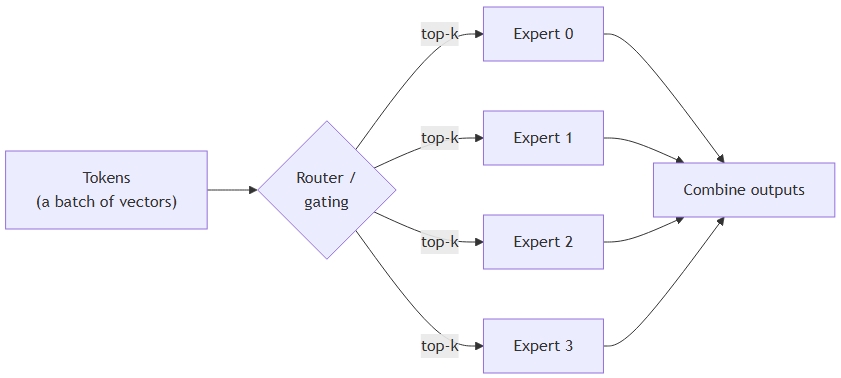
Figure 1: MoE overview: router/gating selects top-k experts per token#
The Consequence for a Compiler: Variable-Size Groups#
Here’s the crucial systems detail. Because the router assigns each token to experts based on the token’s content, the number of tokens that land on each expert is different, and it is only known at runtime. One expert might receive 2,000 tokens this step; its neighbor might receive 50; the split changes with every batch.
If we gather all the tokens routed to the same expert into a contiguous block, an MoE layer becomes:
A stack of token rows, partitioned into
Gcontiguous groups (one per expert), where groupghasm_grows and them_gvalues vary and are runtime-dependent.Each expert
ghas its own weight matrix, so we need to computeoutput_g = tokens_g × W_g, i.e. a matmul of shape[m_g, k] × [k, n].
Figure 2 illustrates groups with unequal sizes: each color represents an expert.
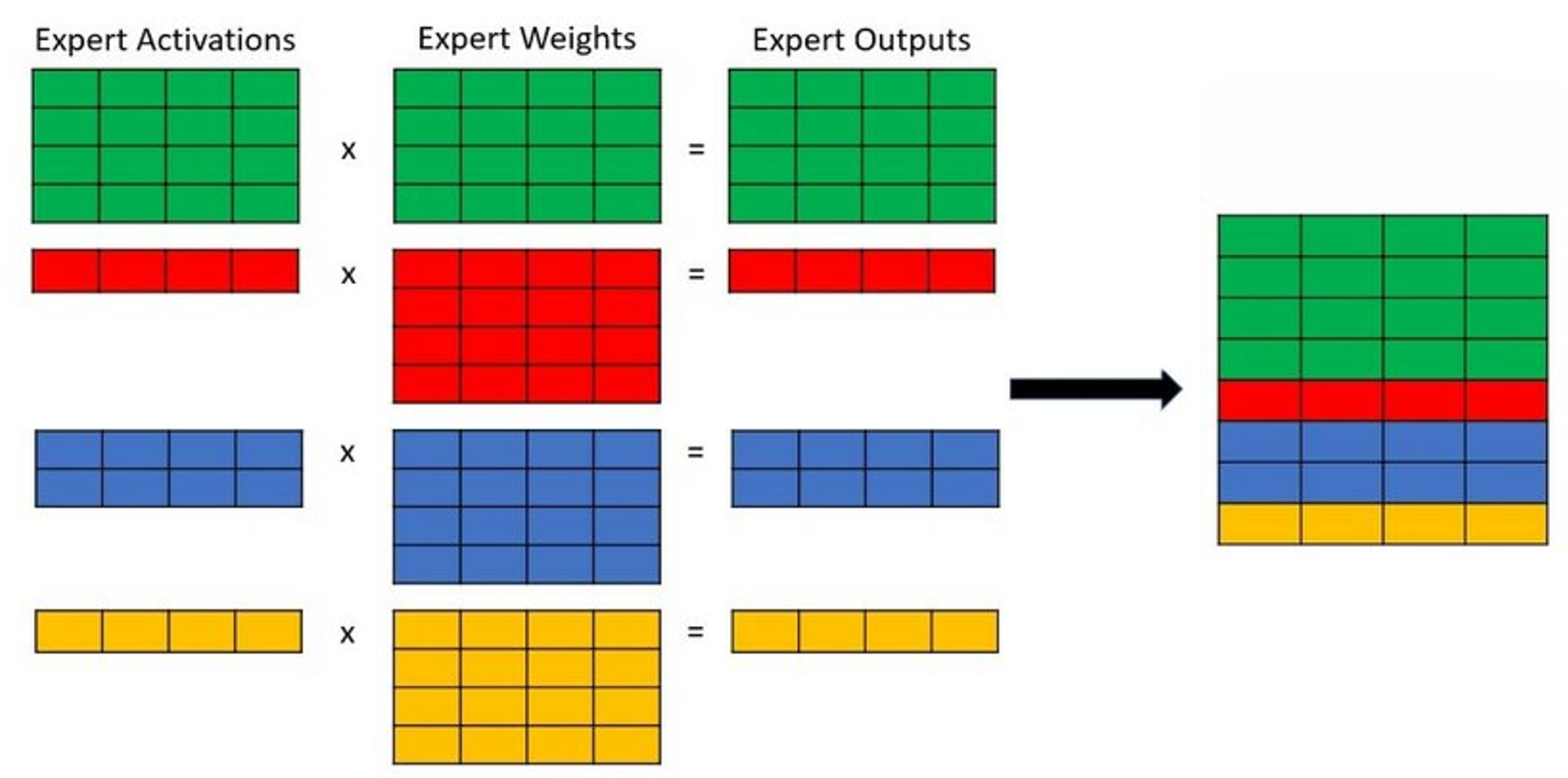
Figure 2: Illustration of MoE experts (each color corresponds to a different expert)#
The mental model to keep for the rest of this post:
An MoE layer is a batch of matmuls whose left-hand-side rows are split into contiguous, variable-size groups.
That “variable-size groups” property is what we call ragged.
The Naive Support, and Why It Hurts: Padded-Dot#
GPUs are well suited to regular, dense shapes. So the naive solution is to force the ragged problem back into a dense one:
Pick a fixed capacity
C(a maximum number of tokens per expert).Pad every expert’s token block up to
Crows.Now every block has the same shape, so we can run one big batched GEMM over
E × [C, k] × [k, n].
Figure 3 illustrates this padding process: every expert’s block is padded to the same
C rows, where the grey padding is compute the GPU performs for nothing.
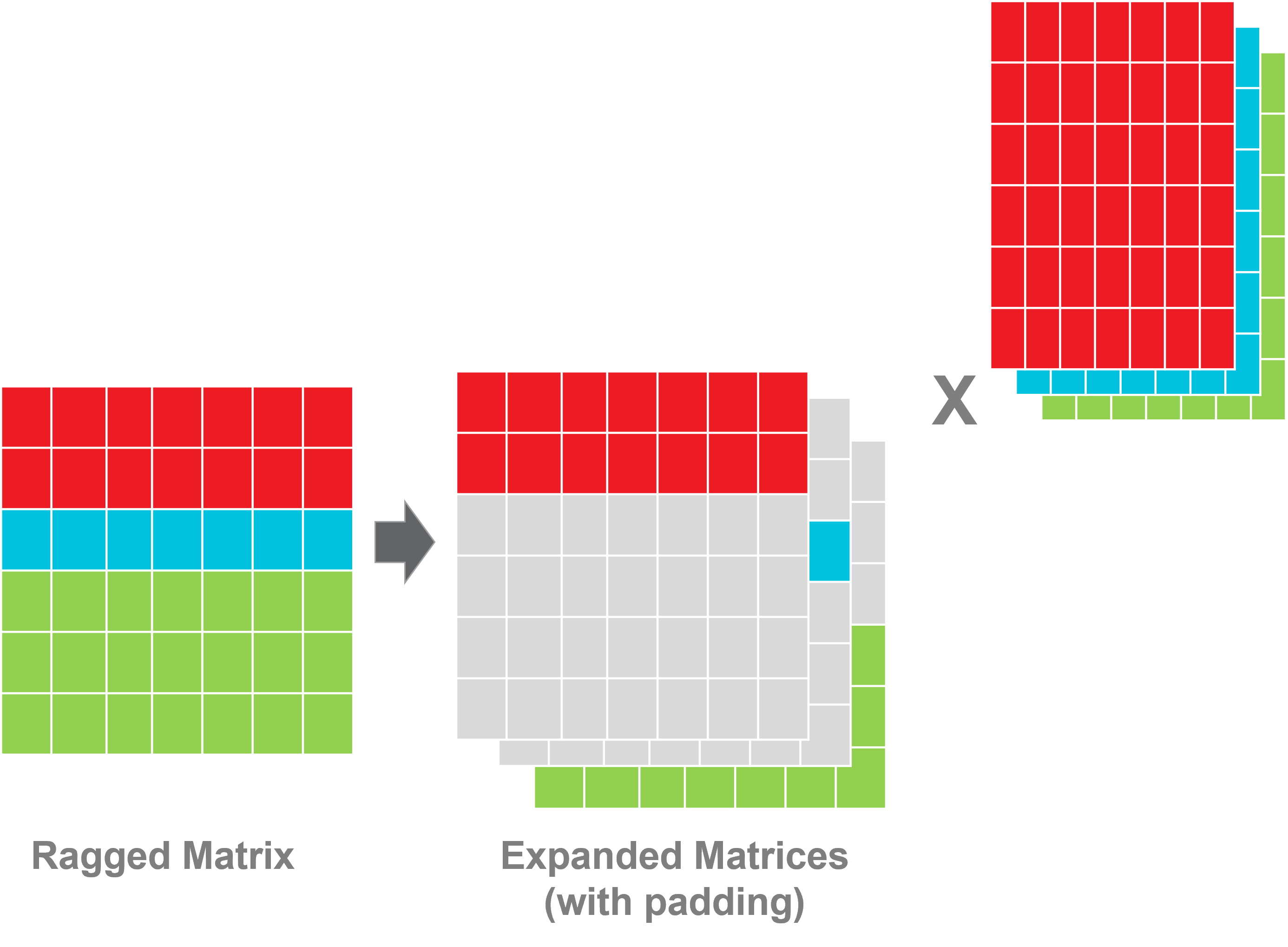
Figure 3: Illustration of padded-dot#
This works, but it is wasteful in two ways:
Wasted compute. Any expert that received fewer than
Ctokens still does a fullC-row matmul; the padding rows are pure overhead.Wasted memory and bandwidth. The compact ragged input has to be expanded into
Epadded matrices, and the outputs have to be compacted again afterwards. Those scatter/gather and pre/post-processing steps cost extra memory and memory traffic.
This “expand into padded matrices” approach is exactly the XLA baseline we’ll compare against later.
The Ragged-Dot Operation#
Rather than having users replace their MoE with a dense problem, JAX lets you describe the ragged
computation directly with ragged_dot.
The basic form:
jax.lax.ragged_dot(lhs, rhs, group_sizes, ...)
with the shapes:
lhsis 2D:[m, k]— all the tokens, stacked, in group order.rhsis 3D:[group, k, n]— one weight matrix per group (per expert).group_sizesis 1D:[group]— how many rows oflhsbelong to each group.the output is 2D.
The group_sizes operand is the key: it is a small vector, known only at
runtime, that partitions the m rows of lhs into contiguous groups. For
example group_sizes = [m_g0, m_g1, m_g2] means the first m_g0 rows are
group 0, the next m_g1 rows are group 1, and so on.
Note that jax.lax.ragged_dot is a JAX-level operation. When the JAX program is
compiled, it is converted into the HLO ragged-dot operation (kRaggedDot),
which is the actual input XLA receives and lowers.
Figure 4 illustrates the operands of a ragged-dot.
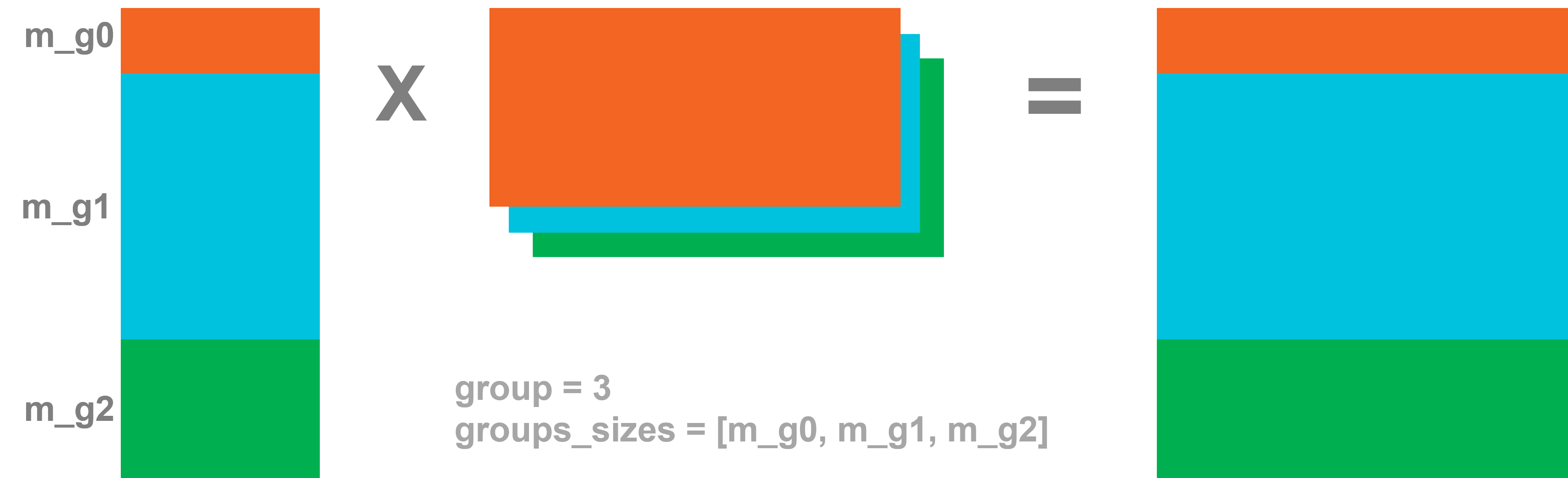
Figure 4: Illustration of ragged-dot#
JAX also offers a more general form:
jax.lax.ragged_dot_general(lhs, rhs, group_sizes, ragged_dimension, ...)
which lets you choose which dimension is the ragged one. That choice yields the three variants listed in Table 1 and drawn in Figure 5:
Table 1: The three ragged-dot variants exposed by jax.lax.ragged_dot_general.
Variant |
Ragged dimension |
What it means |
Group index in output? |
|---|---|---|---|
Non-contracting ( |
the “rows” dimension |
the classic MoE case |
No |
Contracting ( |
the reduction dimension |
groups along the contracted axis |
Yes |
Batch ( |
a batch dimension |
effectively a regular batched GEMM |
— |
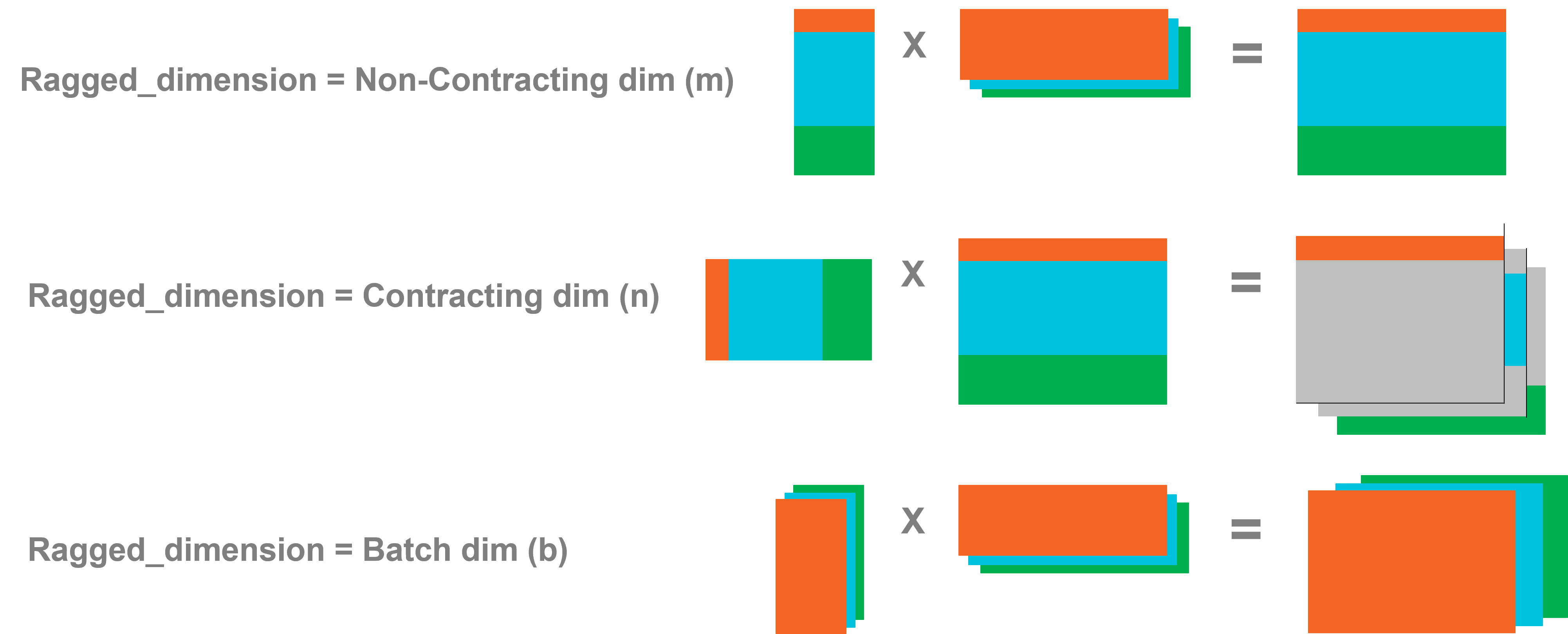
Figure 5: Illustration of generic ragged-dot#
Inside XLA these correspond to the kRaggedDot variants
kRaggedNonContracting, kRaggedContracting, and kRaggedBatch. For MoE,
the one that matters most is non-contracting, where the rows (tokens) are ragged.
Why Group-GEMM Is the Suitable Solution#
Group-GEMM is an API for matrix multiplication that generalizes the usual batched GEMM: instead of requiring every matrix in the batch to share the same shape, it lets each one differ — in size, transposition, activation, and scaling factors. In other words:
Group-GEMM = a set of independent GEMMs of different shapes, computed in a single operation.
That is a perfect match for ragged-dot, as ragged-dot is nothing more than a set of independent GEMMs of different shapes where the pointer to the input data can be calculated from the base pointer of the operand buffer + an offset derived at runtime from the group-size operands.
Hence, Group-GEMM can take care of “unpacking” the ragged
operand and computing all of the per-expert products in one kernel launch, with no padding, as shown in Figure 6.
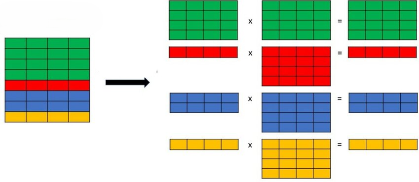
Figure 6: Group-GEMM unpacking the ragged operand into per-group matmuls#
Compared to the padded-dot baseline, this directly removes both costs described in The Naive Support, and Why It Hurts: Padded-Dot:
No padding FLOPs — each group does exactly the work it needs.
No expansion/copies — the compact ragged layout is consumed as-is.
The rest of this post is about the two backends XLA uses to turn ragged-dot into real Group-GEMM for AMD GPUs.
Part 2 — Backend #1: hipBLASLt Group-GEMM (AMD ROCm)#
Overview#
AMD’s hipBLASLt library has supported Group-GEMM since version 1.2.2.
XLA already had a hipBLASLt backend for ordinary dot operations, so the natural move was to extend that existing
backend to also lower ragged-dot down to hipBLASLt Group-GEMM.
Figure 7 shows the lowering path of a plain dot, and Figure 8 the ragged-dot path added alongside it.

Figure 7: Dot op XLA lowering diagram#

Figure 8: Ragged-dot op XLA lowering diagram#
The implementation reuses the existing matmul backend machinery and simply derives a GroupedMatmulPlan class from MatmulPlan, including the additional parameters required to run the hipBLASLt Group-GEMM.
struct GroupedGemmConfig {
  uint64_t m, n, k;
  uint64_t batch_count;
  uint64_t group_count;
  int64_t lhs_leading_dim_stride;
  int64_t rhs_leading_dim_stride;
  int64_t c_leading_dim_stride;
  int64_t output_leading_dim_stride;
  blas::Transpose trans_a, trans_b;
  bool must_swap_operands;
  xla::complex128 alpha;
  double beta;
  blas::DataType type_a, type_b, type_c, type_d;
  int64_t stride_ragged_dim;
  int64_t stride_group_dim;
  int64_t c_stride_ragged_dim;
  int64_t output_stride_ragged_dim;
  // PrecisionConfig-level algorithm
  xla::PrecisionConfig::Algorithm precision_algorithm;
  int64_t compute_precision;
  RaggedDotMode ragged_mode;
  std::optional<blas::ComputationType> compute_type;

  static absl::StatusOr<GroupedGemmConfig> FromProto(
      const xla::GroupedGemmConfigProto& proto);
  xla::GroupedGemmConfigProto ToProto() const;
};

class GroupedMatmulPlan : public gpu::BlasLt::MatmulPlan {
   public:
    friend class BlasLt;

    GroupedMatmulPlan(const BlasLt& blas_lt, const gpu::GroupedGemmConfig& cfg)
        : blas_lt_(blas_lt), cfg_(cfg) {}

    ~GroupedMatmulPlan() override = default;

    absl::Status ExecuteOnStream(
        Stream* stream, const gpu::BlasLt::MemoryArgs& args,
        blas::ProfileResult* profile_result) const override;

    absl::StatusOr<std::vector<MatmulAlgorithm>> GetAlgorithms(
        size_t max_algorithm_count, size_t max_workspace_size) const override;

    absl::Status SetAlgorithm(const MatmulAlgorithm& algorithm) override {...}

   private:
    ...

    const BlasLt& blas_lt_;
    gpu::GroupedGemmConfig cfg_;
    Epilogue epilogue_ = Epilogue::kDefault;
    std::unique_ptr<hipblaslt_ext::GroupedGemm> grouped_gemm_;
    mutable std::optional<hipblasLtMatmulAlgo_t> algorithm_;
    mutable bool algorithm_dirty_ = false;
    mutable DeviceAddressBase saved_address_workspace_{};
    // Saved default activation parameters from hipBLASLt
    int32_t activation_type_ = 0;
    int8_t bias_type_ = 0;
  };  // class GroupedMatmulPlan
(source code available GroupedGemmConfig and GroupedMatmulPlan)
The hipBLASLt Group-GEMM API#
Launching a Group-GEMM with hipBLASLt follows the fixed sequence of steps shown in Figure 9:

Figure 9: hipBLASLt Group-GEMM launch sequence#
The important concept here is user arguments. hipBLASLt describes each individual matmul in the group with its own descriptor — a small structure that says how much data to read and from where: the matmul’s sizes, its input pointers, and its strides. There is one descriptor per matmul, and all of them must live in GPU global memory at the moment the Group-GEMM launches. (See here for more details on the user argument structure definition).
The Compile-Time vs. Runtime Problem#
Here is the central difficulty. XLA is an ahead-of-time compiler: it wants to plan and configure the operation at compile time. But the whole point of ragged-dot is that the group sizes — and therefore each matmul’s dimensions — are only known at runtime. So, we need a way to delay the specification of the matmul’s dimensions to runtime.
Fortunately, hipBLASLt provides a neat trick to bridge the gap. The extension allows the operation sizes (m, n, k, and batch) to be redefined at runtime, in device memory, by modifying the user arguments.
Only one condition must be guaranteed: the total problem
size defined at compile time must be equal to or greater than the sum of the sizes of all the individual GEMMs that are actually executed.
(You can see the documentation for more details on this.)
In XLA, the definition of user arguments is therefore delayed until runtime.
Just before launching the Group-GEMM, XLA executes small update kernels on the GPU that
compute and populate the descriptors with the actual sizes of the groups contained in group_sizes.
These kernels proceed as sketched in Figure 10:

Figure 10: Update kernels: each thread populates one matmul descriptor from group_sizes#
Each thread is responsible for one matmul’s descriptor. It uses a prefix sum (a block-scan) over the group sizes to figure out where its group starts in the packed buffers, computes the correct sizes, strides, scales, and data pointers, and writes them to a shared-memory staging buffer. After a synchronization, all threads cooperatively copy the completed set of descriptors into global memory, where hipBLASLt expects to find them at launch.
Autotuning#
hipBLASLt’s Group-GEMM API can enumerate all the algorithms available for a given problem, and XLA’s autotuner benchmarks them to pick the fastest, as shown in Figure 11:
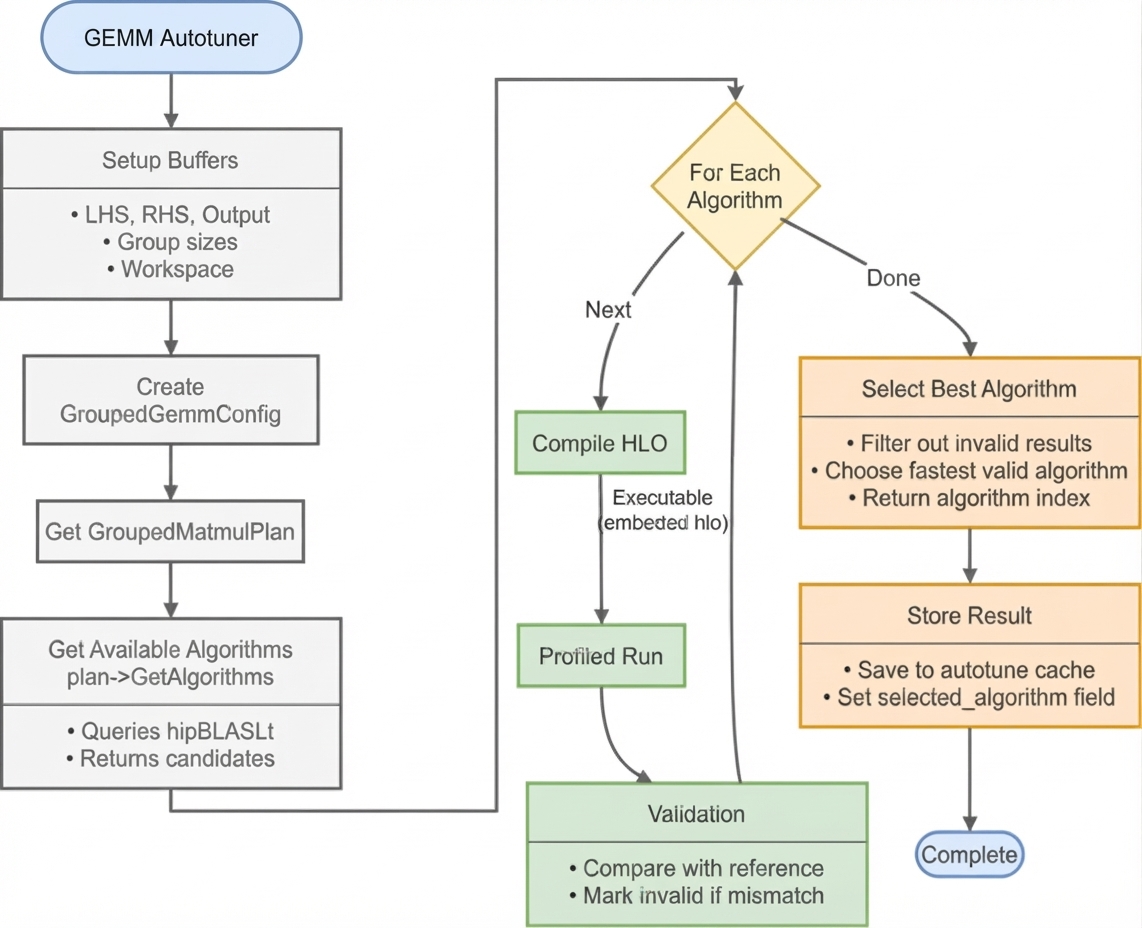
Figure 11: XLA GEMM autotuner#
However, ragged-dot needs one special accommodation. By default, the autotuner profiles candidates on buffers filled with random values. But for
Group-GEMM, group_sizes is not ordinary data: its values are used to compute memory offsets and pointers. Random group sizes would produce invalid offsets and corrupt (or crash) the memory accesses.
To address this problem, the autotuner was enhanced to seed the group_sizes buffer with consistent values before profiling. More specifically, the sum of the group_sizes values must be equal to the
size M of the ragged dimension.
For example, for a ragged dimension of size M = 1024 split across G = 4 groups, the autotuner seeds group_sizes = [256, 256, 256, 256] (256 × 4 = 1024 = M). When M is not divisible by G, the remainder is spread over the first groups (e.g. M = 1002 → [251, 251, 250, 250]). In both cases sum(group_sizes) == M.
Enforcing sum(group_sizes) == M guarantees two things:
In-bounds pointers. Each group’s data pointer is derived from a prefix sum over
group_sizes(group_ptr = base_ptr + prefix_sum(group_sizes)[i] * stride); keeping the sum equal toMensures every derived pointer stays inside the operand buffer.A fully-written output.
ragged-dotallowssum(group_sizes) < M, but then part of the output buffer is left unwritten — during autotuning this would leave uninitialized (garbage) values that make result comparison unreliable. Seeding the sum to exactlyMensures the entire output is written, so profiled candidates can be compared safely.
Part 3 — Backend #2: Triton Ragged-Dot (Portable CUDA + ROCm)#
Motivation#
Even though the hipBLASLt path provides impressive performance (see Part 4 — Performance Evaluation),
it is ROCm-specific and not even available on every AMD GPU target.
On the other hand, Triton is a generic backend that can be lowered to most GPU targets.
In addition, Triton kernels can more easily be fused together, making it a privileged backend for the XLA compiler, which aims to run on any GPU target.
Consequently, we decided to propose a Triton backend as an alternative to efficiently handle the ragged-dot operation in XLA.
In a nutshell, the Triton backend consists of lowering the ragged-dot operation into a Group-GEMM Triton kernel, through XLA’s Triton tiling-and-emission pipeline.
The Compilation Pipeline#
Figure 12 shows the main steps that have been enhanced to enable the lowering of the ragged-dot op:

Figure 12: Triton ragged-dot compilation pipeline#
Backend selection. XLA decides which path serves this
ragged-dot, following a priority order: cuDNN (CUDA) → hipBLASLt (ROCm) → Triton → a default fallback. When the Triton path is chosen, XLA wraps theragged-dotin a custom Triton fusion and seeds it with default tile sizes that the autotuner can later override. Note that the backend selection order is currently fixed by static rules, but the next step is to let the XLA autotuner choose the best backend for each specific problem’s inputs.Support validation. Before committing, XLA checks the
ragged-dotis actually supported: it must be aragged-dotwith exactly one ragged left-hand-side dimension, the tiling-propagation feature must be enabled, and the element types must be supported.
Scheduling. XLA decides how the
ragged-dot’s logical dimensions (M, N, G, K) map onto the GPU grid — which become parallel grid axes (one program per tile, run concurrently) and which stay sequential (a loop inside a program, typically the K reduction).This step includes an M/N-swap heuristic. This heuristic already existed for the ordinary
dot(andscaled_dot) but has been extended forragged-dot. It is therefore useful to briefly recall what it does for a plain GEMM.Plain GEMM. For a regular
LHS[M,K] × RHS[K,N] → out[M,N], the M and N tiles form a 2-D grid that XLA linearizes into a 1-D stream of program IDs. Whichever axis is placed outer varies slowly, and the inner one varies fastest across consecutive programs. The heuristic exploits this to maximize L2 reuse: if the LHS (activations) is smaller in bytes than the RHS (weights), it swaps M and N so that N is traversed slowly — keeping the small LHS tile-row resident in L2 while streaming across the many N tiles. Concretely it comparesByteSizeOf(lhs)againstByteSizeOf(rhs)and, when the LHS is smaller, emits a permutation that swaps the M and N grid axes.Ragged-dot. A ragged-dot is not one big matmul but
Gsmaller ones, so the raw operand byte-sizes are the wrong thing to compare. The ragged version keeps the same mechanism (permute the parallel grid axes before the program-id is delinearized) but changes the decision: it uses the compile-time estimateM_avg = M_total / G— the average number of rows per group — as a proxy for how tall each group’s LHS activation slice really is (the true per-group sizes are only known at runtime).Autotuning. The pipeline generates candidate tiling configurations specialized for ragged-dot and benchmarks them (more on the ragged-specific profiling wrinkle in Autotuning and the
group_sizesSeeding Problem).Emission. Finally, XLA emits the actual Triton kernel for the selected variant.
What the Emitted Triton Kernel Does, per Variant#
Now, let’s take a closer look at the Triton kernels generated to execute the generic ragged-dot operations, which encompass three variants depending on which dimension is the ragged dimension.
As we argued before, the Group-GEMM algorithm is best suited to handle ragged-dot operations.
We therefore generate different kernels for each variant, which all implement the Group-GEMM algorithm but differ in the way they use the group_sizes information to calculate pointer offsets.
The tricky point with a Triton kernel is that each kernel defines the program running on one thread block. Then, the GPU launches a grid of programs (one per output tile); so each program needs to figure out which slice of data it owns, perform the matmul for that slice, and write its output tile. So, what differs between the variants is:
where the raggedness lives,
whether
group_sizesis loaded at all,how the group offset is used.
Note that how these per-tile programs are laid out across the grid is a scheduling decision, not part of the per-program arithmetic above. Two complementary mechanisms shape that layout:
the M/N-swap heuristic from The Compilation Pipeline, which decides which grid axis varies slowly so that the smaller per-group operand stays resident in L2; and
a tile-id remapping in the emitter (specific to the non-contracting/MoE variant), which reorders program IDs so that tiles belonging to the same group run close together, keeping that group’s RHS weight matrix hot in L2 cache. (Note that this optimization was replicated for the ROCm AITER Group-GEMM implementation).
Together these keep each expert’s weights cache-resident while its tiles are being computed.
Non-Contracting (the MoE Case)#

Figure 13: Non-Contracting ragged-dot illustration#
Shape: LHS[M_total, K] × RHS[G, K, N] → out[M_total, N]. The ragged axis
is M (the stacked tokens). Every output row m belongs to exactly one group
g = group(m), and that group selects which weight matrix RHS[g] is used.
The emitted kernel has (conceptually) this signature:
@triton.jit
def ragged_dot_non_contracting(
    lhs_ptr,          # [M_total, K]  all tokens, stacked in group order
    rhs_ptr,          # [G, K, N]     one weight matrix per group (expert)
    out_ptr,          # [M_total, N]  output, same row layout as lhs
    group_sizes_ptr,  # [G]           rows per group; sum == M_total
    M_total, K, N, G,
    BLOCK_M: tl.constexpr, BLOCK_N: tl.constexpr, BLOCK_K: tl.constexpr,
):
    pid_m = tl.program_id(0)      # which M-tile this program owns
    pid_n = tl.program_id(1)      # which N-tile this program owns
    row_start = pid_m * BLOCK_M   # first LHS row of this tile (in [0, M_total))
    ...
The subtle part of the kernel is to “know” which portion of the data the kernel is expected to compute.
Indeed, the program only knows its M-tile position — i.e. which band of BLOCK_M rows of the stacked LHS it is responsible for (row_start = pid_m * BLOCK_M). What it does not directly know is which expert those rows came from, because the group boundaries depend on the runtime group_sizes. To recover the group it runs a prefix sum over group_sizes:
group_sizes         = [ m0, m1,     m2,       … ]
prefix (exclusive)  = [ 0,  m0,     m0+m1,    … ]   # group start rows
prefix (inclusive)  = [ m0, m0+m1,  m0+m1+m2, … ]   # group end rows
The exclusive prefix sum gives the start row of every group; the inclusive
one gives the end row. The program’s group g is simply the group whose
[start, end) interval contains its row_start — i.e. the largest g such that prefix_exclusive[g] <= row_start. From that same table it reads
group_start_row = prefix_exclusive[g], which tells it the offset of its group inside the stacked buffer (needed to address LHS/out correctly, and to mask the partial tile at the group’s boundary).
Table 2 below works through a tiny example — group_sizes = [3, 2, 4] (so M_total = 9) and
BLOCK_M = 3:
Table 2: Worked example of the group lookup for group_sizes = [3, 2, 4] with BLOCK_M = 3.
|
|
falls in group |
|
uses weights |
|---|---|---|---|---|
0 |
0 |
0 (rows 0–2) |
0 |
|
1 |
3 |
1 (rows 3–4) |
3 |
|
2 |
6 |
2 (rows 5–8) |
5 |
|
(When a tile straddles a group boundary, the emitter masks the rows outside the group so each row is only ever attributed to a single expert.)
Per program:
Compute the prefix sum over
group_sizes; from its own M-tile position (row_start = pid_m * BLOCK_M) find which groupgit falls into (the group whose[start, end)row interval containsrow_start) and read that group’s start rowgroup_start_row = prefix_exclusive[g].Use the group index
gto select the matching RHS sliceRHS[g, :, :], i.e. that expert’s weight matrix.Accumulate a tiled dot product over the contraction dimension K (the usual GEMM inner loop), producing an
[BLOCK_M, BLOCK_N]output tile, and write it toout.
group_sizes is loaded — it drives both the group selection and the row
offset. Figure 14 summarizes this program flow.

Figure 14: Non-contracting program: prefix sum selects group g and its RHS weights#
Contracting#
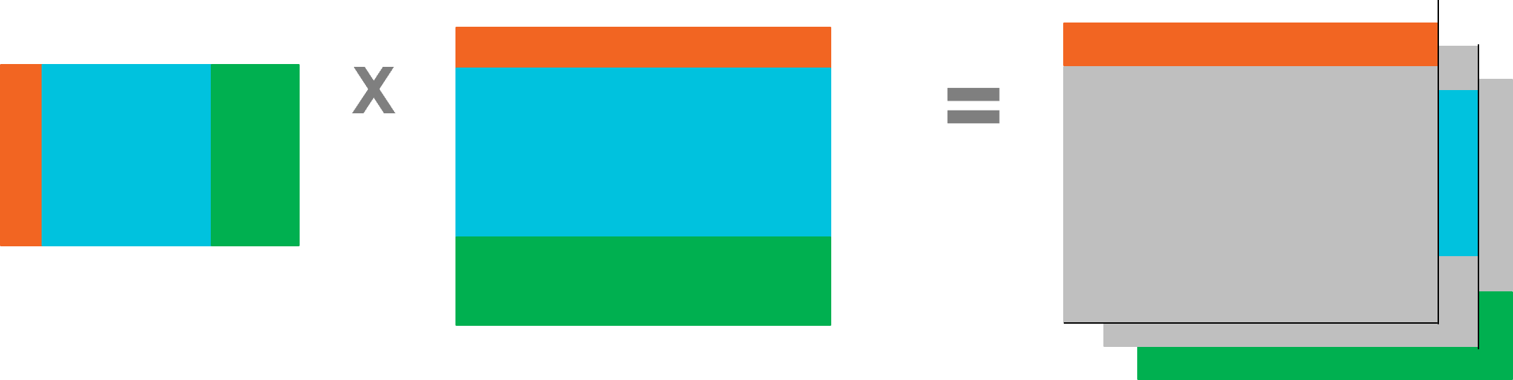
Figure 15: Contracting ragged-dot illustration#
Shape: LHS[M, K_total] × RHS[K_total, N] → out[G, M, N]. The ragged axis is the K (contracted) dimension, and — unlike the non-contracting case — the group index shows up in the output: instead of one contraction over all of K, each group g contributes its own result matrix by reducing only over the slice of the contracted axis that belongs to it.
The emitted kernel has (conceptually) this signature:
@triton.jit
def ragged_dot_contracting(
    lhs_ptr,          # [M, K_total]  contracted axis is ragged
    rhs_ptr,          # [K_total, N]
    out_ptr,          # [G, M, N]     one output matrix per group
    group_sizes_ptr,  # [G]           K-slice size per group; sum == K_total
    M, K_total, N, G,
    BLOCK_M: tl.constexpr, BLOCK_N: tl.constexpr, BLOCK_K: tl.constexpr,
):
    pid_g = tl.program_id(0)      # which group this program owns (→ output slab g)
    pid_m = tl.program_id(1)      # which M-tile
    pid_n = tl.program_id(2)      # which N-tile
    ...
The key structural difference from the non-contracting case is that the group dimension does exist in the output, and that changes how a program finds its group:
For the non-contracting kernel, the group index does not appear in the output shape — all groups write into the same
[M_total, N]buffer, stacked by row. A program is assigned an M-tile (a band of rows) and must find out which group those rows belong to by scanning the prefix sum.For the contracting kernel, the group index is an output dimension (
out[G, M, N]). Each group produces its own[M, N]output, so the groups can simply be distributed over the grid. Consequently, XLA makesGa parallel grid axis, and each program is handed its group directly aspid_g.
To illustrate this, Figure 16 shows the same pool of blocks
under the two kernels. In the non-contracting case a block is placed by its (M-tile, N-tile) position and only afterwards figures out its group g from the prefix sum — so the group is a runtime label, not a launch coordinate. In the contracting case the G axis is part of the launch grid, so each block is born owning a specific group g = pid_g — the groups are literally spread across blocks by the scheduler.
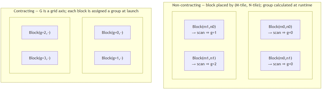
Figure 16: Block placement: non-contracting derives group at runtime; contracting assigns group at launch#
What the program needs from group_sizes is where along K its group’s
slice begins and ends — the ragged K partition is still runtime data. It reads that from the same prefix-sum table:
group_sizes         = [ k0,   k1,      k2,        … ]   # K-rows per group
prefix (exclusive)  = [ 0,    k0,      k0+k1,     … ]   # k_start for each group
prefix (inclusive)  = [ k0,   k0+k1,   k0+k1+k2,  … ]   # k_end   for each group
For its own pid_g, the program reads k_start = prefix_exclusive[pid_g] and k_end = prefix_inclusive[pid_g], then contracts over only [k_start, k_end) of the K axis.
Per program:
Take its group
g = pid_gfrom the grid, and readk_start/k_endfrom the prefix sum overgroup_sizes— this time the offset locates the group’s slice along the contracted axis.Accumulate a partial dot over just that
[k_start, k_end)slice of the contracted axis.Write to
out[g, :, :]— the output position indexed by the groupg.
group_sizes is loaded: it provides the per-group start/end offsets along K.
Figure 17 summarizes this program flow.

Figure 17: Contracting program: group comes from the grid; K-slice from prefix sum#
Batch#

Figure 18: Batch dimension ragged-dot illustration#
Shape: LHS[B, M, K] × RHS[B, K, N] → out[B, M, N] — an ordinary batched
GEMM. The ragged dimension is a batch dimension, but because every batch
element is fully computed there are no data-dependent group offsets to work
out: each program simply owns one (batch, M-tile, N-tile) and does a full
contraction over K.
The emitted kernel has (conceptually) this signature:
@triton.jit
def ragged_dot_batch(
    lhs_ptr,          # [B, M, K]
    rhs_ptr,          # [B, K, N]
    out_ptr,          # [B, M, N]
    B, M, K, N,
    BLOCK_M: tl.constexpr, BLOCK_N: tl.constexpr, BLOCK_K: tl.constexpr,
):
    pid_b = tl.program_id(0)      # which batch element this program owns
    pid_m = tl.program_id(1)      # which M-tile
    pid_n = tl.program_id(2)      # which N-tile
    # no prefix sum: batch index and tile offsets are enough to address the data
    ...
Because the batch index pid_b comes straight from the grid and every batch
element has the same, statically-known shape, the program can compute all of its pointers from pid_b, pid_m, pid_n and the compile-time strides alone. There is no group boundary to discover, so group_sizes is not even loaded here. It influences scheduling only, but not the arithmetic.
Per program:
Take its batch index
b = pid_bfrom the grid (and itspid_m,pid_ntile positions).Accumulate a tiled dot product over K between
LHS[b]andRHS[b].Write the
[BLOCK_M, BLOCK_N]result toout[b, M-tile, N-tile].
group_sizes is not loaded: it is used only as a scheduling hint.
Figure 19 summarizes this program flow.
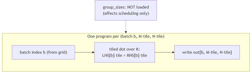
Figure 19: Batch program: batch index from grid; group_sizes not loaded#
Autotuning and the group_sizes Seeding Problem#
This backend runs into the very same issue as the hipBLASLt autotuner in
Autotuning.
During autotuning, candidate kernels run on synthetic input buffers, which
are filled with random bytes by default. That’s harmless for a normal GEMM.
But group_sizes is made of control values that determine loop bounds and
memory offsets.
The fix mirrors the hipBLASLt one: before profiling, the profiler writes
balanced, valid data into the group_sizes buffer — every group gets an equal share of the rows, and the last group absorbs any remainder — guaranteeing the sizes sum exactly to the ragged dimension.
Part 4 — Performance Evaluation#
Every comparison is made against the padded-dot baseline from The Naive Support, and Why It Hurts: Padded-Dot:
the ragged-dot is rewritten into regular dot operations by expanding the ragged input of G groups into G padded matrices, with the associated pre- and post-processing of the input and output matrices. This is the “before” picture that Group-GEMM aims to beat, recalled in Figure 20.
Figure 20: Illustration of padded-dot#
Testbed Characteristics#
The performance evaluations have been performed on two AMD GPU targets, MI300 (gfx942) and MI350 (gfx950). The software configuration was as follows:
Operating System: Ubuntu 22.04
ROCm version: 7.2.4
JAX version: upstream (https://github.com/jax-ml/jax) commit 0eb0f676ba22b15b9dfe29518ab0d40277b7138d
XLA version: ROCm (https://github.com/ROCm/xla) branch pr/ragged-dot-6-e2e-tests (upstream commit e5d008bb03d9b133b0881daf3d108adea8e6625b + ragged-dot Triton support commits)
MaxText version: ROCm (https://github.com/ROCm/maxtext) commit fb25ae8c850fa2b57dd5eb7ebfbe399f08534e69
Note that ROCm version 7.2.4 only offers Group-GEMM support for bf16 on MI300. Support for bf16 on MI350 was not yet available when this blog post was written.
The ragged-dot Triton backend is not enabled by default and must be explicitly enabled using the following flag xla_gpu_experimental_triton_ragged_dot=true.
Furthermore, note that this backend is only supported with the Triton experimental tiling feature.
As a consequence, the flag xla_gpu_experimental_enable_tiling_propagation=true must be set alongside the xla_gpu_experimental_triton_ragged_dot flag.
Last, the default Triton autotuning is not yet fine-tuned for ragged-dot, so exhaustive search was used for the evaluation xla_gpu_exhaustive_tiling_search=true.
Use Case: MoE Model Training Using MaxText#
MaxText is a high-performance,
highly scalable, open-source LLM library and reference implementation written in
Python/JAX. Because it is written on top of JAX, its MoE layers ultimately lower to
JAX primitives — and, on the sparse path, to the jax.lax.ragged_dot op that the
Group-GEMM backends described above accelerate. This makes MaxText an ideal
framework in which to evaluate the new ragged-dot backends on realistic MoE models.
Two MoE Modes: Drop vs. Dropless#
Before diving into how MaxText runs the expert FFNs, it helps to recall that there are two ways of handling the per-expert token counts of an MoE layer — and the choice between them is an accuracy/efficiency trade-off.
Drop mode. Each expert is given a fixed capacity
expert_capacity(expert_capacity = ceil(tokens_per_batch / E) × capacity_factor). Tokens routed beyond an expert’s capacity are simply dropped (they skip the FFN and contribute nothing), and under-filled experts are padded up toexpert_capacity. This keeps every expert’s matmul a regular, statically-shaped[expert_capacity, K] × [K, N], which is hardware-friendly, but it wastes FLOPs on the padding of under-filled experts and loses information on the dropped tokens of over-filled ones.Dropless mode. No token is ever dropped and no capacity padding is introduced: every routed (token, expert) pair is computed exactly. This preserves the full model quality, but it requires handling the ragged, data-dependent per-expert sizes — either by physically gathering tokens per expert into one ragged matmul (the block-sparse formulation introduced by MegaBlocks [Gale et al., 2022], which is exactly the
ragged-dot/Group-GEMM path this post is about), or by running a full dense compute over all tokens and masking afterwards.
Figure 21 illustrates the buffers the two modes produce.
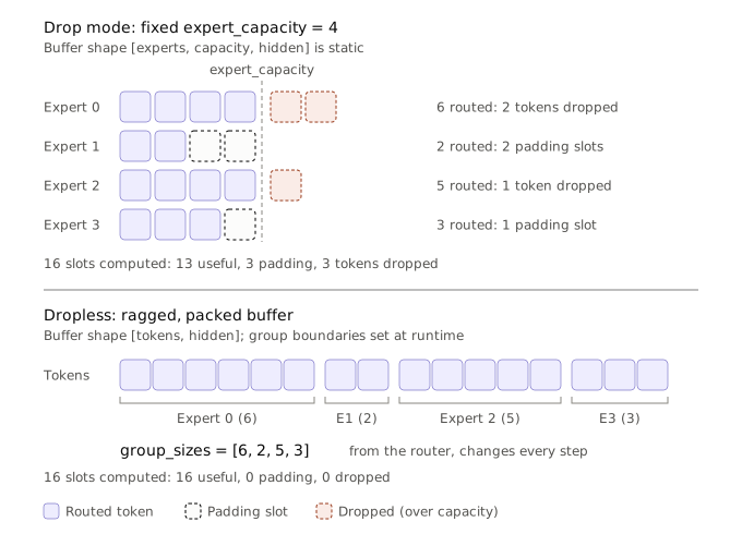
Figure 21: Drop vs. dropless MoE modes: drop mode pads/truncates each expert to a fixed capacity, while dropless mode keeps the compact, ragged per-expert buffers with no padding and no dropping.#
The rest of this section looks at how MaxText realizes these two modes through its three concrete compute paths. For a complementary, MaxText-focused deep dive into the dropless MoE path and its optimization, see the AMD ROCm blog Dropless MoE in MaxText.
The Three MoE Compute Paths in MaxText#
Before diving into the models, it is worth noticing that ragged-dot is only one
of several ways to run the expert FFNs and combine their outputs.
If you look at the MaxText framework, it exposes three distinct MoE compute
paths — two of them implement the dropless mode (the sparse / ragged-dot path
and the dense mask-and-combine path), while one implements the drop mode (the
capacity-based dense dispatch/combine path). The ragged-dot/Group-GEMM work
described so far powers just one of the two dropless paths.
All three share the same front-end — a router (gating network) picks, for every token, its top-k experts and a weight per selected expert:
# gate_logits: [B, S, E]
top_k_weights, top_k_indices = jax.lax.top_k(gate_logits, num_experts_per_tok)  # [B, S, k]
However, they differ in the way the selected (token, expert) pairs are turned into matmuls, and in the pre-/post-processing that surrounds those matmuls.
From a user’s point of view, two config knobs allow choosing the path:
sparse_matmul—Truepicks the sparse (ragged-dot) path (the dropless, block-sparse formulation of the MoE computation);Falsepicks one of the two dense paths.capacity_factor— inside the dense path,> 0enables token dropping (fixed per-expert capacity);<= 0keeps it dropless.
Figure 22 shows how these two knobs select a path.
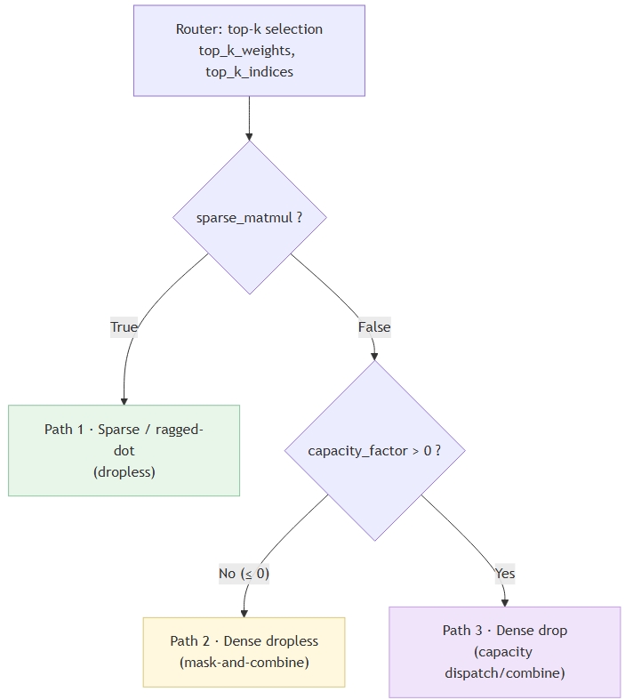
Figure 22: MoE path selection: sparse_matmul and capacity_factor pick one of three paths#
Table 3 summarizes the trade-offs before we look at each path in detail:
Table 3: The three MaxText MoE compute paths and their trade-offs.
Path 1 — Sparse (ragged-dot) |
Path 2 — Dense dropless |
Path 3 — Dense drop |
|
|---|---|---|---|
config |
|
|
|
expert op |
|
dense per-expert einsum over all tokens |
dense capacity-padded batched einsum |
pre-processing |
permute (sort tokens by expert) + |
none (broadcast all tokens to all experts) |
build dispatch mask (one-hot into capacity slots), drop overflow |
post-processing |
un-permute (scatter back) + weighted sum |
weighted combine ( |
combine mask gathers from capacity slots back to tokens |
compute cost |
≈ |
≈ |
≈ |
drops tokens? |
no |
no |
yes (overflow beyond |
padding |
none |
none (but full dense compute) |
per-expert capacity padding |
Path 1 — Sparse / Ragged-Dot (Dropless)#
Selected by sparse_matmul = True. This is the path that generates jax.lax.ragged_dot ops which are then lowered by XLA. The idea is to physically gather the tokens by expert
so that the expert FFNs become one big ragged matmul.
Pre-processing — permute. The router’s top_k_indices are used to sort all
M = B·S·top_k token-copies into contiguous per-expert groups, and a bincount
produces the group_sizes vector (real routed counts, summing to M):
# permute(): sort token rows by their assigned expert, count per-expert sizes
sorted_selected_experts = jnp.argsort(jnp.ravel(selected_experts))
sorted_inputs = _sort_activations(replicated_inputs, sorted_selected_experts)  # [M, K]
group_sizes  = jnp.bincount(jnp.ravel(selected_experts), length=num_experts)   # [E], sums to M
Compute — Group-GEMM. The gathered tokens and the per-expert weights feed
directly into jax.lax.ragged_dot, which can be later lowered to hipBLASLt / Triton Group-GEMM by XLA.
# gmm(): the expert FFN as a single ragged/group matmul
out = jax.lax.ragged_dot(lhs=sorted_inputs,        # [M, K]  tokens, grouped by expert
                         rhs=w,                     # [E, K, N] expert weights
                         group_sizes=group_sizes,   # [E]
                         preferred_element_type=dtype)
Post-processing — un-permute. The results are scattered back to the original token order and the top-k contributions are summed with the router weights:
# unpermute(): invert the sort, then weighted-combine the top-k expert outputs
unsorted = _sort_activations(out, jnp.argsort(sorted_selected_experts))
output   = jnp.einsum("BKE,BK -> BE", unsorted.reshape(-1, top_k, N), top_k_weights)
The whole path is summarized in Figure 23.

Figure 23: Path 1 (sparse): permute → ragged_dot (Group-GEMM) → un-permute#
Cost: only the real routed rows are ever multiplied — compute is
≈ M × K × N with no padding and no dropping. So, regarding the matrix multiplication itself, this path with Group-GEMM backends provides the most efficient solution.
However, we have to pay for the sort/scatter (permute/un-permute) which is needed to put the data in a form that can be processed by the Group-GEMM backends.
Path 2 — Dense Dropless (Mask-and-Combine)#
Selected by sparse_matmul = False and capacity_factor ≤ 0. In this path, there is no
gather at all: every token is sent through every expert, and the router
weights (zero for non-selected experts) mask out the unwanted results at the end.
Pre-processing — none (beyond turning top-k into a dense [B,S,E] weight
matrix, 0 where an expert was not selected):
weights = reshape_and_update_weights(top_k_weights, top_k_indices) # [B,S,E], 0 off-selection
Compute — full dense einsums. Each expert processes the entire token batch:
# up / gate: every token × every expert
layer_w0 = jnp.einsum("BSM,EMH -> BSEH", inputs, w0_kernel)   # [B,S,E,H]
layer_w1 = jnp.einsum("BSM,EMH -> BSEH", inputs, w1_kernel)
inter    = activation(layer_w0) * layer_w1
# down
inter    = jnp.einsum("BSEH,EHM -> BSEM", inter, wo_kernel)   # [B,S,E,M]
Post-processing — weighted combine. The router weights collapse the expert axis, keeping only each token’s selected experts:
output = jnp.einsum("BSEM,BSE -> BSM", inter, weights) # [B,S,M]
The whole path is summarized in Figure 24.

Figure 24: Path 2 (dense dropless): all tokens × all experts, then weighted combine#
Cost: dropless and permutation-free, but compute is ≈ E × (B·S) × K × N —
every token pays for every expert, so it scales with the full expert count.
This is simple and hardware-friendly (plain dense matmuls, no ragged handling) but
becomes prohibitively expensive as E grows.
Path 3 — Dense Drop (Capacity Dispatch/Combine)#
Selected by sparse_matmul = False and capacity_factor > 0. This is the
classic fixed-capacity MoE: each expert gets a static slot of
C = ceil(tokens_per_batch / E) × capacity_factor rows; tokens beyond C are dropped.
Pre-processing — dispatch mask (with dropping). generate_masks builds a
one-hot dispatch_mask that assigns each kept (token, expert) pair to a capacity
slot and truncates any overflow:
expert_capacity = ceil(tokens_per_batch / num_experts) * capacity_factor
# ... one-hot into [B,S,E,C]; positions past `expert_capacity` are dropped ...
dispatch_mask, combine_mask = generate_masks(top_k_indices, weights)
Compute — capacity-padded batched einsum. Tokens are scattered into the
[E, B, C, M] capacity buffer, run through the experts, and the result stays in
capacity layout:
dispatch = jnp.einsum("BSM,BSEC -> EBCM", inputs, dispatch_mask)     # scatter to slots
layer_w0 = jnp.einsum("EBCM,EMH -> EBCH", dispatch, w0_kernel)       # up/gate
inter    = activation(layer_w0) * jnp.einsum("EBCM,EMH -> EBCH", dispatch, w1_kernel)
inter    = jnp.einsum("EBCH,EHM -> EBCM", inter, wo_kernel)          # down
Post-processing — combine mask. The combine_mask gathers each token’s
outputs back from its capacity slots and applies the router weights:
output = jnp.einsum("EBCM,BSEC -> BSM", inter, combine_mask) # gather back to tokens
The whole path is summarized in Figure 25.

Figure 25: Path 3 (dense drop): capacity dispatch → experts → combine mask#
Cost: compute is ≈ E × C × K × N. Because C is fixed, under-filled experts
waste FLOPs on padding rows and over-filled experts drop tokens (an accuracy
trade-off). The capacity buffer also inflates the activation memory.
What About Performance?#
In theory, the ragged-dot/Group-GEMM path:
vs. Path 2 (dense dropless) — Group-GEMM computes only the routed rows (
M × K × N) instead of every-token-times-every-expert (E × B·S × K × N), so it wins by a factor that grows with the number of experts — at the cost of the permute/un-permute sort.vs. Path 3 (dense drop) — Group-GEMM needs no capacity, no padding, and drops no tokens: it consumes the compact
[M, K]layout with realgroup_sizes, avoiding both the wasted-padding FLOPs and the accuracy hit of dropping, while also using less activation memory.
In other words, Group-GEMM keeps the dropless quality of Path 2 with a compute/memory profile close to the ideal (only real work, no padding), trading it for a sort and a ragged-aware kernel. But the remaining question is: how fast is the Group-GEMM kernel itself compared to these dense alternatives on real hardware?
MaxText Models#
We evaluated the performance improvement achieved by the new ragged-dot backends using MaxText MoE models.
The evaluated models are described below, and their configurations are given in
Table 4 (MI300) and Table 5 (MI350):
“Routing-heavy” vs. “compute-heavy”: each MoE layer spends time on (a) the expert GEMM itself (
ragged_dot, ≈ M[tokens] × K[emb] × N[moe_mlp]) and (b) routing — gating top-k selection plus the token permute/sort/scatter that builds thenum_expertsragged groups and the un-permute afterwards. A config is routing-heavy when (b) dominates: this happens with smallbase_moe_mlp_dim(N) (each expert GEMM does little arithmetic) and/or many experts (more small groups → more launch + scatter/gather overhead, lower per-group occupancy). The opposite corner — large N, few experts — is compute-heavy (big dense expert GEMMs dominate, routing negligible).
mixtral-8x7b (MI300 & MI350) — The baseline dense-attention MoE microbenchmark
(emb 6144, 24 layers, 32 experts top-4, dot_product attention, no MLA). Used to
profile the raw ragged-dot expert GEMM without MLA complexity, at 8-way FSDP,
seq 3072, grad-accum 1. The MI300 and MI350 configurations have identical shapes.
It is the primary knob-sweep model for tile sizes and backend (hipBLASLt vs. Triton vs. the default baseline).
mixtral-8x7b-large (MI300 & MI350) — A deliberately enlarged mixtral variant (emb/K 8192, moe_mlp/N 28672, 32 layers, 64 experts top-8) that grows both the expert-GEMM K/N dims and the number of ragged groups. Runs 8-way FSDP at seq 4096, grad-accum 8. It is the compute-heavy corner of the sweep — big, dense expert GEMMs with many groups — used to measure ragged-dot throughput at high arithmetic intensity and to check that larger tiles fit within HBM (192 GB HBM3 / 288 GB HBM3e).
deepseek2-16b (MI300 & MI350) — A scaled-down DeepSeek-V2 test (emb 2048,
27 layers, 64 experts top-6, 2 shared experts) that keeps the real MLA attention and
deepseek decoder block. It validates the ragged-dot + MLA + YARN-RoPE code path
cheaply, running autodetected FSDP, grad-accum 4, seq 512. Shared experts add a dense
side-path alongside the routed experts, exercising the mixed dense/sparse MLP.
deepseek3-test (MI300 & MI350) — A tiny DeepSeek-V3 CI proxy (emb 512) that
keeps the deepseek block + MLA attention but shrinks everything else. On MI300 it is
cut to 16 layers / 32 experts (dense mlp 4096); on MI350 it retains the full 61-layer /
256-expert topology with the tiny emb 512. Runs autodetected FSDP, grad-accum 4,
seq 512 — a fast functional check of the ragged-dot + MLA path rather than a perf run.
deepseek3-671b-reduced (MI300 & MI350) — A perf-representative slice of the flagship 671B DeepSeek-V3: it preserves the real expert-GEMM shapes (K/emb 7168, N/moe_mlp 2048, MLA) but cuts to 4 layers / 32 experts so it fits on 8 GPUs. Because FSDP can’t hold the full model it is expert-parallel (EP=8, 4 experts/GPU, FSDP off), grad-accum 8, seq 512. This makes the per-expert GEMM timing representative of the true 671B while keeping the run tractable.
gemma4-26b (MI300 only) — Gemma-4 26B MoE (emb 2816, 30 layers, 128 experts
top-8, 1 shared) with the gemma4 decoder block and standard dot_product attention.
Small base_moe_mlp_dim (704) means many narrow expert GEMMs, stressing per-group
launch/routing overhead rather than raw FLOPs. Runs autodetected FSDP, seq 1024,
grad-accum 4 — a good test for many-small-experts ragged-dot
efficiency on the 192 GB HBM3 gfx942 platform.
qwen3-30b-a3b (MI300 & MI350) — Qwen3 MoE (emb 2048, 48 layers, 128 experts
top-8, qwen3_moe block, QK-norm) with a very small expert width
(base_moe_mlp_dim 768). Like gemma4 it is dominated by many thin expert GEMMs and
routing overhead rather than arithmetic intensity. MI300 and MI350 use identical shapes
(autodetected FSDP, seq 1024, grad-accum 4). A
lightweight but routing-heavy ragged-dot workload.
qwen3-235b-a22b (MI350 only) — Large Qwen3 MoE (emb 4096, 94 layers, 128 experts top-8, moe_mlp 1536). The deep 94-layer stack combined with 128 experts makes it the heaviest routing/attention workload in the tables; it runs 8-way FSDP, seq 2048, grad-accum 16. Sequence length and layer depth push activation memory, so remat and FSDP are essential to fit — a scale/depth stress test for ragged-dot.
llama4-17b-16e (MI350 only) — Llama-4 17B, 16-expert, top-1 routing (each token → a single expert) with wide experts (moe_mlp 8192) and a shared expert. This combination makes it the compute-heavy corner: a few large, dense expert GEMMs where the padded-dot baseline already wastes little, so Group-GEMM has limited headroom to improve on it. Runs autodetected FSDP, seq 1024, grad-accum 4.
MI300 (MI300X, gfx942, 192 GB HBM3, 8× GPU)#
Table 4: MaxText MoE model configurations evaluated on MI300.
Model (config) |
emb_dim (K) |
moe_mlp_dim (N) |
mlp_dim |
layers |
experts |
top-k |
shared |
attn |
seq len |
grad-accum |
parallelism (FSDP / EP / TP) |
|---|---|---|---|---|---|---|---|---|---|---|---|
mixtral-8x7b |
6144 |
20480 |
20480 |
24 |
32 |
4 |
– |
dot |
3072 |
1 |
8 / 1 / 1 |
mixtral-8x7b-large |
8192 |
28672 |
28672 |
32 |
64 |
8 |
– |
dot |
4096 |
8 |
8 / 1 / 1 |
deepseek2-16b |
2048 |
1408 |
5632 |
27 |
64 |
6 |
2 |
MLA |
512 |
4 |
auto / 1 / 1 |
deepseek3-test |
512 |
512 |
4096 |
16 |
32 |
8 |
1 |
MLA |
512 |
4 |
auto / 1 / 1 |
deepseek3-671b-reduced |
7168 |
2048 |
18432 |
4 |
32 |
8 |
1 |
MLA |
512 |
8 |
1 / 8 / 1 |
gemma4-26b |
2816 |
704 |
2112 |
30 |
128 |
8 |
1 |
dot |
1024 |
4 |
auto / 1 / 1 |
qwen3-30b-a3b |
2048 |
768 |
768 |
48 |
128 |
8 |
– |
dot |
1024 |
4 |
auto / 1 / 1 |
MI350-Class (gfx950, 288 GB HBM3e, 8× GPU)#
Table 5: MaxText MoE model configurations evaluated on MI350.
Model (config) |
emb_dim (K) |
moe_mlp_dim (N) |
mlp_dim |
layers |
experts |
top-k |
shared |
attn |
seq len |
grad-accum |
parallelism (FSDP / EP / TP) |
|---|---|---|---|---|---|---|---|---|---|---|---|
mixtral-8x7b |
6144 |
20480 |
20480 |
24 |
32 |
4 |
– |
dot |
3072 |
1 |
8 / 1 / 1 |
mixtral-8x7b-large |
8192 |
28672 |
28672 |
32 |
64 |
8 |
– |
dot |
4096 |
8 |
8 / 1 / 1 |
deepseek2-16b |
2048 |
1408 |
5632 |
27 |
64 |
6 |
2 |
MLA |
512 |
4 |
auto / 1 / 1 |
deepseek3-test |
512 |
512 |
18432 |
61 |
256 |
8 |
1 |
MLA |
512 |
4 |
auto / 1 / 1 |
deepseek3-671b-reduced |
7168 |
2048 |
18432 |
4 |
32 |
8 |
1 |
MLA |
512 |
8 |
1 / 8 / 1 |
qwen3-30b-a3b |
2048 |
768 |
768 |
48 |
128 |
8 |
– |
dot |
1024 |
4 |
auto / 1 / 1 |
qwen3-235b-a22b |
4096 |
1536 |
1536 |
94 |
128 |
8 |
– |
dot |
2048 |
16 |
8 / 1 / 1 |
llama4-17b-16e |
5120 |
8192 |
8192 |
48 |
16 |
1 |
1 |
dot |
1024 |
4 |
auto / 1 / 1 |
Legend:
emb_dim (K)= expert-GEMM contraction dimmoe_mlp_dim (N)= expert-GEMM output dimattn= attention type (MLA = Multi-head Latent Attention — DeepSeek’s low-rank compressed KV attention)parallelism=ici_fsdp_parallelism / ici_expert_parallelism / ici_tensor_parallelism, i.e. FSDP (Fully Sharded Data Parallel — params/grads/optimizer sharded across GPUs) / EP (Expert Parallel — MoE experts distributed across GPUs) / TP (Tensor Parallel — individual matmuls split across GPUs)auto=-1(autodetects available GPUs).
Micro-Benchmark#
In order to evaluate the performance increase provided by the new backends for the ragged-dot operations, we isolated the ragged-dot operations executed in the MaxText models mentioned above and created a synthetic micro-benchmark that “replays” these operations alone. This micro-benchmark is written at the JAX level (so it evaluates the whole compilation pipeline), runs the identified ragged-dot ops 50 times (after a 10-run warm-up), and calculates the average execution time over these 50 runs. As the hipBLASLt Group-GEMM backend is only available for the bf16 datatype on MI300, we chose to show only numbers for this target in this blog post.
From an MoE Layer to 6 Ragged-Dot Classes#
An MoE expert block in MaxText is built from two projections — an up/gate projection (wi) and a down projection (wo) — and each of those has to be differentiated, producing a data gradient (dgrad) and a weight gradient (wgrad) in the backward pass.
When you enumerate every ragged-dot XLA emits across the forward + backward
pass, they collapse into exactly 6 structural classes. Two operations belong
to the same class if and only if their operands share the same rank (number of dimensions) and the same contracting / ragged / group dimension numbers, and the output has the same rank and layout. However, the sizes (M, K, N, E) may differ.
In the following, we use the notation given in Table 6:
Table 6: Notation used to describe the ragged-dot classes.
symbol |
meaning |
|---|---|
|
ragged token dimension = |
|
expert-GEMM contraction / embedding dim ( |
|
expert-GEMM output dim ( |
|
number of experts ( |
|
|
The M (token) axis is the ragged axis: it is partitioned into E groups, one per expert, and dtype is bfloat16 throughout.
The six classes are listed in Table 7:
Table 7: The six structural ragged-dot classes emitted across the forward and backward pass.
class |
role |
lhs |
rhs |
out |
contract (lhs,rhs) |
rhs_group |
|---|---|---|---|---|---|---|
|
fwd gate/up |
|
|
|
|
|
|
fwd down |
|
|
|
|
|
|
dgrad up |
|
|
|
|
|
|
dgrad down |
|
|
|
|
|
|
wgrad up |
|
|
|
|
|
|
wgrad down |
|
|
|
|
|
All classes are bfloat16, with lhs_ragged_dimensions = {0} and
group_sizes = int32[E].
The forward classes (
fwd_wi,fwd_wo) are the plainjax.lax.ragged_dotform —inputs[M,K] × w[E,K,N] → out[M,N]for the gate/up projection, andinterm[M,N] × w[E,N,K] → out[M,K]for the down projection.The dgrad classes (
dgrad_wi,dgrad_wo) contract the weight’s output-feature axis (rhs_contracting = {2}), so they require the explicitragged_dot_generalform with custom dimension numbers.The wgrad classes (
wgrad_wi,wgrad_wo) are[M,·] × [M,·] → [E,·,·]Group-GEMMs that contract the ragged token axis and produce one weight-gradient slab per expert (emptyrhs_group_dimensions).
For example, fwd_wi — the gate/up projection — is simply:
import jax.numpy as jnp
from jax import lax

lhs = jnp.zeros((M, K), jnp.bfloat16)          # tokens
rhs = jnp.zeros((E, K, N), jnp.bfloat16)       # expert weights
                                               # group_sizes: int32[E], sums to M
out = lax.ragged_dot(lhs, rhs, group_sizes,    # -> [M, N]
                     preferred_element_type=jnp.bfloat16)
while a weight-gradient such as wgrad_wi needs the general form with explicit
dimension numbers:
# a[M,K] × b[M,N] -> w[E,K,N]; contract the ragged M axis, group on the output
wgrad_dn = lax.RaggedDotDimensionNumbers(
    dot_dimension_numbers=(((0,), (0,)), ((), ())),
    lhs_ragged_dimensions=(0,),
    rhs_group_dimensions=(),        # empty -> grouped output on E
)
out = lax.ragged_dot_general(lhs, rhs, group_sizes,   # -> [E, K, N]
                             ragged_dot_dimension_numbers=wgrad_dn,
                             preferred_element_type=jnp.bfloat16)
Fixing group_sizes Deterministically#
In real training the per-expert token counts are data-dependent — they come out of the router and change every step. For a reproducible benchmark we instead use a balanced / uniform partition: every expert receives M // E tokens, and the remainder M mod E is spread one extra token per group across the first M mod E experts, so that sum(group_sizes) == M exactly:
base = M // E                      # tokens per expert (floor)
rem  = M - base * E                # leftover to distribute (0 <= rem < E)
gs = np.full((E,), base, np.int32)
gs[:rem] += 1                      # first `rem` experts get one extra
group_sizes = jnp.asarray(gs)      # int32[E], sums to M
This gives each expert ≈ M/E rows. Real routing is typically less balanced, which tends to lower the achieved TFLOP/s for the per-group backends.
Results#
For each model variant we measure the runtime of all the 6 classes on each backend (default padded-dot baseline, triton, and hip).
The resulting speedups over the baseline are shown in Figure 26.
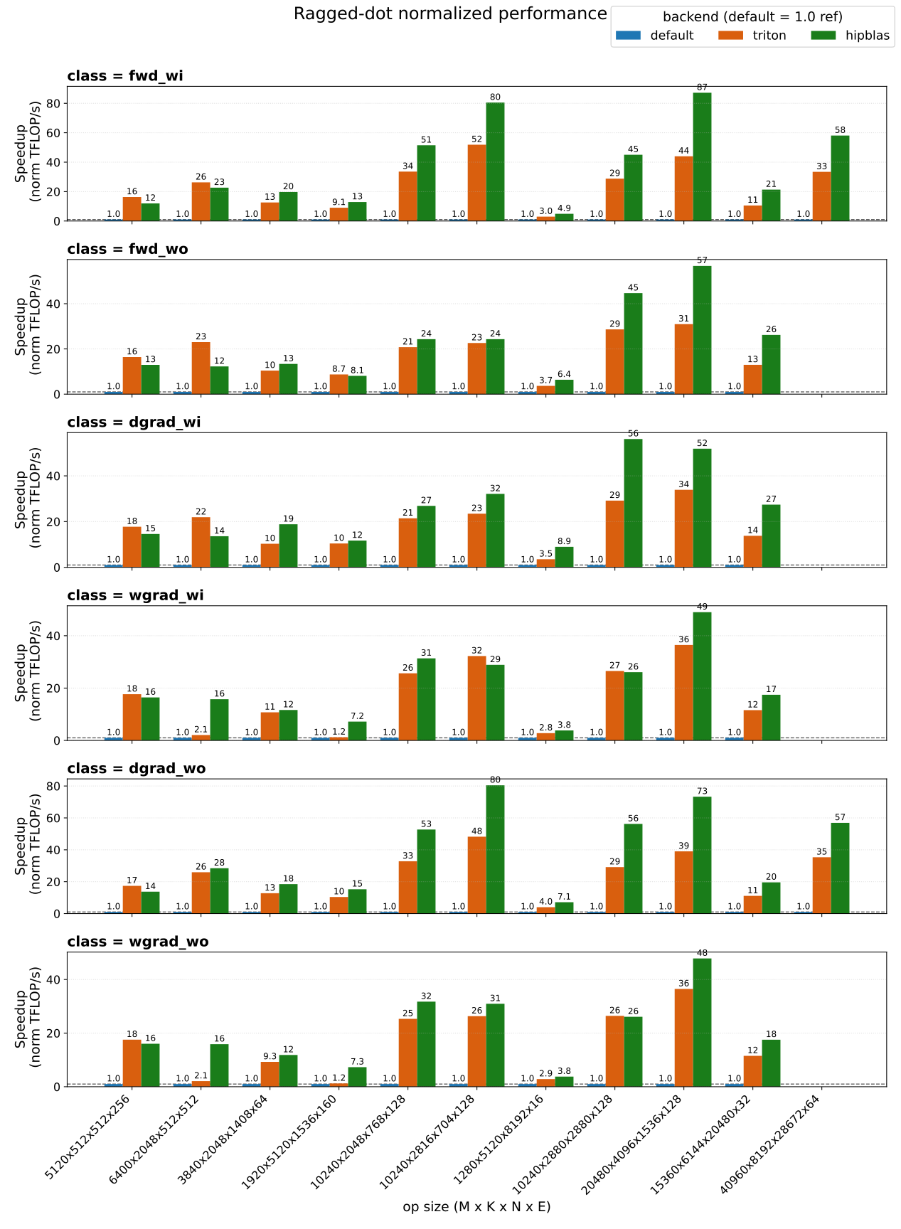
Figure 26: Ragged-dot micro-benchmark speedup#
The full per-class TFLOP/s results for every measured shape are provided in Table 12 of the Appendix: Micro-Benchmark Full Results.
Performance of MaxText MoE Models#
Performance#
Now, let’s consider the overall performance improvement for the whole model train step. Note that in this section, the shown performance is the median value over training steps 5 to 10. The results are reported in Figure 27 and Table 8 for MI300, and in Figure 28 and Table 9 for MI350.
MI300#
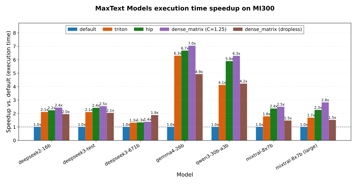
Figure 27: MaxText models execution time speedup on MI300#
Table 8: MaxText MoE model training-step performance on MI300.
Model |
Emb Dim |
Experts |
Exp/Tok |
Layers |
total_weights |
Backend |
execution time (s) |
TFLOP/s/device |
Tokens/s/device |
Speedup |
|---|---|---|---|---|---|---|---|---|---|---|
deepseek2-16b |
2048 |
64 |
6 |
27 |
15.706B |
default |
3.946 |
7.744 |
519.018 |
1.00x |
deepseek2-16b |
2048 |
64 |
6 |
27 |
15.706B |
triton |
1.867 |
16.369 |
1097.136 |
2.11x |
deepseek2-16b |
2048 |
64 |
6 |
27 |
15.706B |
hip |
1.761 |
17.348 |
1162.700 |
2.24x |
deepseek2-16b |
2048 |
64 |
6 |
27 |
15.706B |
dense_matrix |
1.617 |
18.895 |
1266.397 |
2.44x |
deepseek2-16b |
2048 |
64 |
6 |
27 |
15.706B |
dense_matrix_dropless |
2.018 |
15.143 |
1014.919 |
1.96x |
deepseek3-test |
512 |
256 |
8 |
61 |
15.851B |
default |
5.758 |
10.910 |
355.653 |
1.00x |
deepseek3-test |
512 |
256 |
8 |
61 |
15.851B |
triton |
2.732 |
22.995 |
749.610 |
2.11x |
deepseek3-test |
512 |
256 |
8 |
61 |
15.851B |
hip |
2.373 |
26.470 |
862.896 |
2.43x |
deepseek3-test |
512 |
256 |
8 |
61 |
15.851B |
dense_matrix |
2.261 |
27.780 |
905.610 |
2.55x |
deepseek3-test |
512 |
256 |
8 |
61 |
15.851B |
dense_matrix_dropless |
2.806 |
22.387 |
729.808 |
2.05x |
deepseek3-671b |
7168 |
32 |
8 |
4 |
7.415B |
default |
0.575 |
141.236 |
7126.279 |
1.00x |
deepseek3-671b |
7168 |
32 |
8 |
4 |
7.415B |
triton |
0.436 |
186.151 |
9392.514 |
1.32x |
deepseek3-671b |
7168 |
32 |
8 |
4 |
7.415B |
hip |
0.429 |
189.228 |
9547.763 |
1.34x |
deepseek3-671b |
7168 |
32 |
8 |
4 |
7.415B |
dense_matrix |
0.414 |
196.070 |
9893.003 |
1.39x |
deepseek3-671b |
7168 |
32 |
8 |
4 |
7.415B |
dense_matrix_dropless |
0.305 |
265.880 |
13415.345 |
1.89x |
gemma4-26b |
2816 |
128 |
8 |
30 |
25.233B |
default |
20.531 |
4.751 |
199.507 |
1.00x |
gemma4-26b |
2816 |
128 |
8 |
30 |
25.233B |
triton |
3.257 |
29.950 |
1257.783 |
6.30x |
gemma4-26b |
2816 |
128 |
8 |
30 |
25.233B |
hip |
3.073 |
31.737 |
1332.846 |
6.68x |
gemma4-26b |
2816 |
128 |
8 |
30 |
25.233B |
dense_matrix |
2.914 |
33.474 |
1405.770 |
7.05x |
gemma4-26b |
2816 |
128 |
8 |
30 |
25.233B |
dense_matrix_dropless |
4.163 |
23.430 |
983.947 |
4.93x |
qwen3-30b-a3b |
2048 |
128 |
8 |
48 |
30.532B |
default |
20.676 |
3.855 |
198.105 |
1.00x |
qwen3-30b-a3b |
2048 |
128 |
8 |
48 |
30.532B |
triton |
5.013 |
15.897 |
817.004 |
4.12x |
qwen3-30b-a3b |
2048 |
128 |
8 |
48 |
30.532B |
hip |
3.505 |
22.740 |
1168.655 |
5.90x |
qwen3-30b-a3b |
2048 |
128 |
8 |
48 |
30.532B |
dense_matrix |
3.287 |
24.246 |
1246.054 |
6.29x |
qwen3-30b-a3b |
2048 |
128 |
8 |
48 |
30.532B |
dense_matrix_dropless |
4.896 |
16.278 |
836.600 |
4.22x |
mixtral-8x7b |
4096 |
8 |
2 |
32 |
46.703B |
default |
5.044 |
48.057 |
609.025 |
1.00x |
mixtral-8x7b |
4096 |
8 |
2 |
32 |
46.703B |
triton |
2.817 |
86.045 |
1090.451 |
1.79x |
mixtral-8x7b |
4096 |
8 |
2 |
32 |
46.703B |
hip |
2.128 |
113.903 |
1443.498 |
2.37x |
mixtral-8x7b |
4096 |
8 |
2 |
32 |
46.703B |
dense_matrix |
2.015 |
120.291 |
1524.461 |
2.50x |
mixtral-8x7b |
4096 |
8 |
2 |
32 |
46.703B |
dense_matrix_dropless |
3.405 |
71.187 |
902.164 |
1.48x |
mixtral-8x7b (large) |
4096 |
8 |
2 |
32 |
46.703B |
default |
52.107 |
50.128 |
628.859 |
1.00x |
mixtral-8x7b (large) |
4096 |
8 |
2 |
32 |
46.703B |
triton |
30.822 |
84.744 |
1063.120 |
1.69x |
mixtral-8x7b (large) |
4096 |
8 |
2 |
32 |
46.703B |
hip |
22.940 |
113.863 |
1428.421 |
2.27x |
mixtral-8x7b (large) |
4096 |
8 |
2 |
32 |
46.703B |
dense_matrix |
18.438 |
141.662 |
1777.156 |
2.83x |
mixtral-8x7b (large) |
4096 |
8 |
2 |
32 |
46.703B |
dense_matrix_dropless |
34.163 |
76.458 |
959.171 |
1.53x |
MI350#
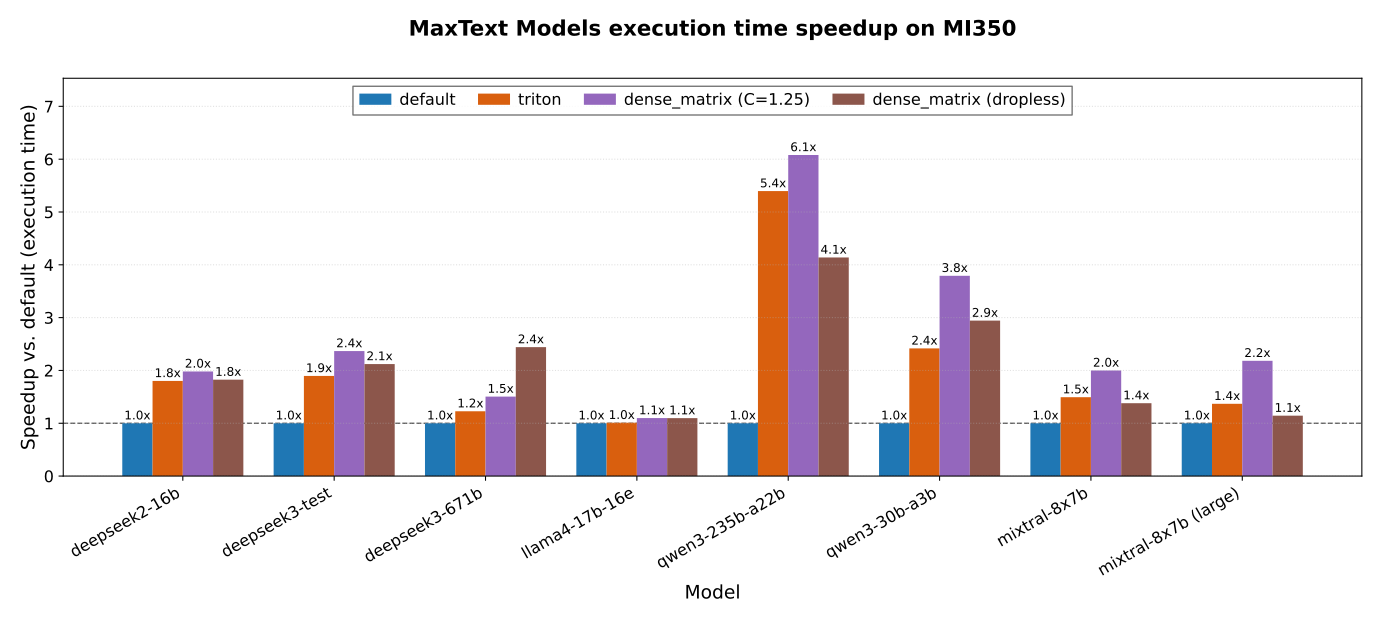
Figure 28: MaxText models execution time speedup on MI350#
Table 9: MaxText MoE model training-step performance on MI350.
Model |
Emb Dim |
Experts |
Exp/Tok |
Layers |
total_weights |
Backend |
execution time (s) |
TFLOP/s/device |
Tokens/s/device |
Speedup |
|---|---|---|---|---|---|---|---|---|---|---|
deepseek2-16b |
2048 |
64 |
6 |
27 |
15.706B |
default |
2.581 |
11.840 |
793.547 |
1.00x |
deepseek2-16b |
2048 |
64 |
6 |
27 |
15.706B |
triton |
1.433 |
21.316 |
1428.675 |
1.80x |
deepseek2-16b |
2048 |
64 |
6 |
27 |
15.706B |
dense_matrix |
1.303 |
23.451 |
1571.765 |
1.98x |
deepseek2-16b |
2048 |
64 |
6 |
27 |
15.706B |
dense_matrix_dropless |
1.414 |
21.603 |
1447.888 |
1.83x |
deepseek3-test |
512 |
256 |
8 |
61 |
15.851B |
default |
4.208 |
14.929 |
486.677 |
1.00x |
deepseek3-test |
512 |
256 |
8 |
61 |
15.851B |
triton |
2.220 |
28.302 |
922.617 |
1.90x |
deepseek3-test |
512 |
256 |
8 |
61 |
15.851B |
dense_matrix |
1.778 |
35.344 |
1152.180 |
2.37x |
deepseek3-test |
512 |
256 |
8 |
61 |
15.851B |
dense_matrix_dropless |
1.984 |
31.662 |
1032.149 |
2.12x |
deepseek3-671b |
7168 |
32 |
8 |
4 |
7.415B |
default |
0.459 |
176.907 |
8926.120 |
1.00x |
deepseek3-671b |
7168 |
32 |
8 |
4 |
7.415B |
triton |
0.374 |
216.782 |
10938.067 |
1.23x |
deepseek3-671b |
7168 |
32 |
8 |
4 |
7.415B |
dense_matrix |
0.305 |
266.230 |
13433.032 |
1.50x |
deepseek3-671b |
7168 |
32 |
8 |
4 |
7.415B |
dense_matrix_dropless |
0.188 |
432.514 |
21823.103 |
2.44x |
llama4-17b-16e |
5120 |
16 |
1 |
48 |
107.770B |
default |
10.249 |
39.299 |
399.631 |
1.00x |
llama4-17b-16e |
5120 |
16 |
1 |
48 |
107.770B |
triton |
10.157 |
39.655 |
403.258 |
1.01x |
llama4-17b-16e |
5120 |
16 |
1 |
48 |
107.770B |
dense_matrix |
9.337 |
43.138 |
438.671 |
1.10x |
llama4-17b-16e |
5120 |
16 |
1 |
48 |
107.770B |
dense_matrix_dropless |
9.344 |
43.108 |
438.372 |
1.10x |
qwen3-235b-a22b |
4096 |
128 |
8 |
4 |
11.196B |
default |
22.025 |
14.110 |
1487.731 |
1.00x |
qwen3-235b-a22b |
4096 |
128 |
8 |
4 |
11.196B |
triton |
4.082 |
76.132 |
8027.089 |
5.40x |
qwen3-235b-a22b |
4096 |
128 |
8 |
4 |
11.196B |
dense_matrix |
3.623 |
85.785 |
9044.923 |
6.08x |
qwen3-235b-a22b |
4096 |
128 |
8 |
4 |
11.196B |
dense_matrix_dropless |
5.322 |
58.391 |
6156.577 |
4.14x |
qwen3-30b-a3b |
2048 |
128 |
8 |
48 |
30.532B |
default |
9.696 |
8.220 |
422.434 |
1.00x |
qwen3-30b-a3b |
2048 |
128 |
8 |
48 |
30.532B |
triton |
4.012 |
19.863 |
1020.834 |
2.42x |
qwen3-30b-a3b |
2048 |
128 |
8 |
48 |
30.532B |
dense_matrix |
2.557 |
31.166 |
1601.701 |
3.79x |
qwen3-30b-a3b |
2048 |
128 |
8 |
48 |
30.532B |
dense_matrix_dropless |
3.294 |
24.197 |
1243.551 |
2.94x |
mixtral-8x7b |
4096 |
8 |
2 |
32 |
46.703B |
default |
2.863 |
84.681 |
1073.164 |
1.00x |
mixtral-8x7b |
4096 |
8 |
2 |
32 |
46.703B |
triton |
1.917 |
126.458 |
1602.606 |
1.49x |
mixtral-8x7b |
4096 |
8 |
2 |
32 |
46.703B |
dense_matrix |
1.432 |
169.318 |
2145.780 |
2.00x |
mixtral-8x7b |
4096 |
8 |
2 |
32 |
46.703B |
dense_matrix_dropless |
2.075 |
116.814 |
1480.395 |
1.38x |
mixtral-8x7b (large) |
4096 |
8 |
2 |
32 |
46.703B |
default |
29.188 |
89.489 |
1122.641 |
1.00x |
mixtral-8x7b (large) |
4096 |
8 |
2 |
32 |
46.703B |
triton |
21.327 |
122.475 |
1536.450 |
1.37x |
mixtral-8x7b (large) |
4096 |
8 |
2 |
32 |
46.703B |
dense_matrix |
13.376 |
195.272 |
2449.693 |
2.18x |
mixtral-8x7b (large) |
4096 |
8 |
2 |
32 |
46.703B |
dense_matrix_dropless |
25.522 |
102.344 |
1283.910 |
1.14x |
The performance numbers confirm that the new Group-GEMM based backends for
jax.lax.ragged_dotoperations provide a significant speedup for MoE models. As expected, thehipBLASLtbackend is faster than the Triton one; however, both offer very interesting speedups. That said, we also notice that the dense matrix (drop case) approach outperforms theragged-dotpath for all the tested models. Indeed, as GPUs are optimized for regular computation, the pure matrix multiplication was expected to be faster than Group-GEMM. However, we might have expected that the extra computation due to the padding would result in a larger slowdown, making theragged-dotapproach faster. But this is not the case, for two main reasons:
the capacity is relatively low (1.25), which means that the padding is relatively small, but potentially a significant number of tokens could be dropped;
the pre-processing to put the data in shape for the
ragged-dotbackend is expensive. Consequently, for the relatively small models evaluated, the time overhead introduced by the pre-processing cancels out the benefit of the Group-GEMM performing only useful multiplications. But with larger models the pre-processing overhead could be better balanced against the matmul efficiency, making theragged-dotGroup-GEMM backends attractive.
Memory Savings#
The memory-usage figures below were extracted directly from the log traces
emitted by MaxText during each training run. MaxText reports, per run, the
peak device memory footprint (broken down into total and temporary/scratch
memory), which we collected for each backend (default, triton, hip) and
diffed against the default padded-dot baseline to obtain the savings shown.
They are reported in Figure 29 and Table 10 for MI300, and in Figure 30 and Table 11 for MI350.
MI300#
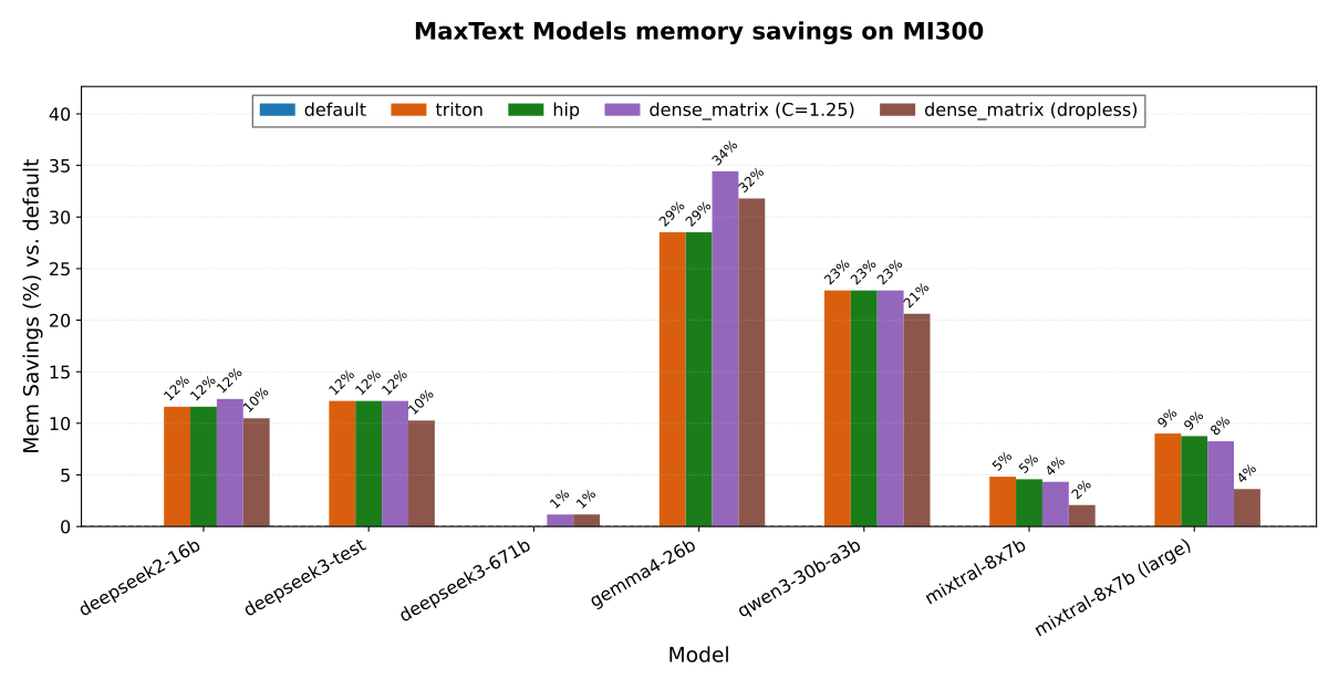
Figure 29: MaxText models memory savings on MI300 (higher is better)#
Table 10: MaxText MoE model peak memory footprint on MI300.
Model |
Emb Dim |
Experts |
Exp/Tok |
Layers |
total_weights |
Backend |
Total Mem (GB) |
Temp Mem (GB) |
Mem Savings (GB) |
Temp Savings (GB) |
|---|---|---|---|---|---|---|---|---|---|---|
deepseek2-16b |
2048 |
64 |
6 |
27 |
15.706B |
default |
26.7 |
15.7 |
0.0 (0.0%) |
0.0 (0.0%) |
deepseek2-16b |
2048 |
64 |
6 |
27 |
15.706B |
triton |
23.6 |
12.6 |
3.1 (11.6%) |
3.1 (19.7%) |
deepseek2-16b |
2048 |
64 |
6 |
27 |
15.706B |
hip |
23.6 |
12.6 |
3.1 (11.6%) |
3.1 (19.7%) |
deepseek2-16b |
2048 |
64 |
6 |
27 |
15.706B |
dense_matrix (capacity 1.25) |
23.4 |
12.5 |
3.3 (12.4%) |
3.2 (20.4%) |
deepseek2-16b |
2048 |
64 |
6 |
27 |
15.706B |
dense_matrix_dropless |
23.9 |
13.0 |
2.8 (10.5%) |
2.7 (17.2%) |
deepseek3-test |
512 |
256 |
8 |
61 |
15.851B |
default |
26.3 |
15.2 |
0.0 (0.0%) |
0.0 (0.0%) |
deepseek3-test |
512 |
256 |
8 |
61 |
15.851B |
triton |
23.1 |
12.0 |
3.2 (12.2%) |
3.2 (21.1%) |
deepseek3-test |
512 |
256 |
8 |
61 |
15.851B |
hip |
23.1 |
12.0 |
3.2 (12.2%) |
3.2 (21.1%) |
deepseek3-test |
512 |
256 |
8 |
61 |
15.851B |
dense_matrix (capacity 1.25) |
23.1 |
12.0 |
3.2 (12.2%) |
3.2 (21.1%) |
deepseek3-test |
512 |
256 |
8 |
61 |
15.851B |
dense_matrix_dropless |
23.6 |
12.6 |
2.7 (10.3%) |
2.6 (17.1%) |
deepseek3-671b |
7168 |
32 |
8 |
4 |
7.415B |
default |
8.6 |
3.4 |
0.0 (0.0%) |
0.0 (0.0%) |
deepseek3-671b |
7168 |
32 |
8 |
4 |
7.415B |
triton |
8.6 |
3.4 |
0.0 (0.0%) |
0.0 (0.0%) |
deepseek3-671b |
7168 |
32 |
8 |
4 |
7.415B |
hip |
8.6 |
3.4 |
0.0 (0.0%) |
0.0 (0.0%) |
deepseek3-671b |
7168 |
32 |
8 |
4 |
7.415B |
dense_matrix (capacity 1.25) |
8.5 |
3.4 |
0.1 (1.2%) |
0.0 (0.0%) |
deepseek3-671b |
7168 |
32 |
8 |
4 |
7.415B |
dense_matrix_dropless |
8.5 |
3.4 |
0.1 (1.2%) |
0.0 (0.0%) |
gemma4-26b |
2816 |
128 |
8 |
30 |
25.233B |
default |
61.0 |
43.3 |
0.0 (0.0%) |
0.0 (0.0%) |
gemma4-26b |
2816 |
128 |
8 |
30 |
25.233B |
triton |
43.6 |
26.0 |
17.4 (28.5%) |
17.3 (40.0%) |
gemma4-26b |
2816 |
128 |
8 |
30 |
25.233B |
hip |
43.6 |
26.0 |
17.4 (28.5%) |
17.3 (40.0%) |
gemma4-26b |
2816 |
128 |
8 |
30 |
25.233B |
dense_matrix (capacity 1.25) |
40.0 |
22.3 |
21.0 (34.4%) |
21.0 (48.5%) |
gemma4-26b |
2816 |
128 |
8 |
30 |
25.233B |
dense_matrix_dropless |
41.6 |
23.9 |
19.4 (31.8%) |
19.4 (44.8%) |
qwen3-30b-a3b |
2048 |
128 |
8 |
48 |
30.532B |
default |
57.7 |
36.4 |
0.0 (0.0%) |
0.0 (0.0%) |
qwen3-30b-a3b |
2048 |
128 |
8 |
48 |
30.532B |
triton |
44.5 |
23.2 |
13.2 (22.9%) |
13.2 (36.3%) |
qwen3-30b-a3b |
2048 |
128 |
8 |
48 |
30.532B |
hip |
44.5 |
23.2 |
13.2 (22.9%) |
13.2 (36.3%) |
qwen3-30b-a3b |
2048 |
128 |
8 |
48 |
30.532B |
dense_matrix (capacity 1.25) |
44.5 |
23.2 |
13.2 (22.9%) |
13.2 (36.3%) |
qwen3-30b-a3b |
2048 |
128 |
8 |
48 |
30.532B |
dense_matrix_dropless |
45.8 |
24.5 |
11.9 (20.6%) |
11.9 (32.7%) |
mixtral-8x7b |
4096 |
8 |
2 |
32 |
46.703B |
default |
120.2 |
54.9 |
0.0 (0.0%) |
0.0 (0.0%) |
mixtral-8x7b |
4096 |
8 |
2 |
32 |
46.703B |
triton |
114.4 |
49.1 |
5.8 (4.8%) |
5.8 (10.6%) |
mixtral-8x7b |
4096 |
8 |
2 |
32 |
46.703B |
hip |
114.7 |
49.5 |
5.5 (4.6%) |
5.4 (9.8%) |
mixtral-8x7b |
4096 |
8 |
2 |
32 |
46.703B |
dense_matrix (capacity 1.25) |
115.0 |
49.7 |
5.2 (4.3%) |
5.2 (9.5%) |
mixtral-8x7b |
4096 |
8 |
2 |
32 |
46.703B |
dense_matrix_dropless |
117.7 |
52.5 |
2.5 (2.1%) |
2.4 (4.4%) |
mixtral-8x7b (large) |
4096 |
8 |
2 |
32 |
46.703B |
default |
79.9 |
47.2 |
0.0 (0.0%) |
0.0 (0.0%) |
mixtral-8x7b (large) |
4096 |
8 |
2 |
32 |
46.703B |
triton |
72.7 |
40.1 |
7.2 (9.0%) |
7.1 (15.0%) |
mixtral-8x7b (large) |
4096 |
8 |
2 |
32 |
46.703B |
hip |
72.9 |
40.2 |
7.0 (8.8%) |
7.0 (14.8%) |
mixtral-8x7b (large) |
4096 |
8 |
2 |
32 |
46.703B |
dense_matrix (capacity 1.25) |
73.3 |
40.7 |
6.6 (8.3%) |
6.5 (13.8%) |
mixtral-8x7b (large) |
4096 |
8 |
2 |
32 |
46.703B |
dense_matrix_dropless |
77.0 |
44.4 |
2.9 (3.6%) |
2.8 (5.9%) |
MI350#
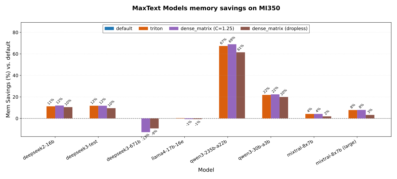
Figure 30: MaxText models memory savings on MI350 (higher is better)#
Table 11: MaxText MoE model peak memory footprint on MI350.
Model |
Emb Dim |
Experts |
Exp/Tok |
Layers |
total_weights |
Backend |
Total Mem (GB) |
Temp Mem (GB) |
Mem Savings (GB) |
Temp Savings (GB) |
|---|---|---|---|---|---|---|---|---|---|---|
deepseek2-16b |
2048 |
64 |
6 |
27 |
15.706B |
default |
26.7 |
15.7 |
0.0 (0.0%) |
0.0 (0.0%) |
deepseek2-16b |
2048 |
64 |
6 |
27 |
15.706B |
triton |
23.7 |
12.7 |
3.0 (11.2%) |
3.0 (19.1%) |
deepseek2-16b |
2048 |
64 |
6 |
27 |
15.706B |
dense_matrix (capacity 1.25) |
23.5 |
12.5 |
3.2 (12.0%) |
3.2 (20.4%) |
deepseek2-16b |
2048 |
64 |
6 |
27 |
15.706B |
dense_matrix_dropless |
23.9 |
13.0 |
2.8 (10.5%) |
2.7 (17.2%) |
deepseek3-test |
512 |
256 |
8 |
61 |
15.851B |
default |
26.3 |
15.2 |
0.0 (0.0%) |
0.0 (0.0%) |
deepseek3-test |
512 |
256 |
8 |
61 |
15.851B |
triton |
23.2 |
12.2 |
3.1 (11.8%) |
3.0 (19.7%) |
deepseek3-test |
512 |
256 |
8 |
61 |
15.851B |
dense_matrix (capacity 1.25) |
23.2 |
12.1 |
3.1 (11.8%) |
3.1 (20.4%) |
deepseek3-test |
512 |
256 |
8 |
61 |
15.851B |
dense_matrix_dropless |
23.8 |
12.8 |
2.5 (9.5%) |
2.4 (15.8%) |
deepseek3-671b |
7168 |
32 |
8 |
4 |
7.415B |
default |
8.6 |
3.4 |
0.0 (0.0%) |
0.0 (0.0%) |
deepseek3-671b |
7168 |
32 |
8 |
4 |
7.415B |
triton |
8.6 |
3.4 |
0.0 (0.0%) |
0.0 (0.0%) |
deepseek3-671b |
7168 |
32 |
8 |
4 |
7.415B |
dense_matrix (capacity 1.25) |
9.7 |
4.5 |
-1.1 (-12.8%) |
-1.1 (-32.4%) |
deepseek3-671b |
7168 |
32 |
8 |
4 |
7.415B |
dense_matrix_dropless |
9.4 |
4.2 |
-0.8 (-9.3%) |
-0.8 (-23.5%) |
llama4-17b-16e |
5120 |
16 |
1 |
48 |
107.770B |
default |
170.5 |
95.2 |
0.0 (0.0%) |
0.0 (0.0%) |
llama4-17b-16e |
5120 |
16 |
1 |
48 |
107.770B |
triton |
170.0 |
94.7 |
0.5 (0.3%) |
0.5 (0.5%) |
llama4-17b-16e |
5120 |
16 |
1 |
48 |
107.770B |
dense_matrix (capacity 1.25) |
171.6 |
96.3 |
-1.1 (-0.6%) |
-1.1 (-1.2%) |
llama4-17b-16e |
5120 |
16 |
1 |
48 |
107.770B |
dense_matrix_dropless |
171.6 |
96.3 |
-1.1 (-0.6%) |
-1.1 (-1.2%) |
qwen3-235b-a22b |
4096 |
128 |
8 |
4 |
11.196B |
default |
74.7 |
66.9 |
0.0 (0.0%) |
0.0 (0.0%) |
qwen3-235b-a22b |
4096 |
128 |
8 |
4 |
11.196B |
triton |
24.4 |
16.5 |
50.3 (67.3%) |
50.4 (75.3%) |
qwen3-235b-a22b |
4096 |
128 |
8 |
4 |
11.196B |
dense_matrix (capacity 1.25) |
23.2 |
15.4 |
51.5 (68.9%) |
51.5 (77.0%) |
qwen3-235b-a22b |
4096 |
128 |
8 |
4 |
11.196B |
dense_matrix_dropless |
28.8 |
21.0 |
45.9 (61.4%) |
45.9 (68.6%) |
qwen3-30b-a3b |
2048 |
128 |
8 |
48 |
30.532B |
default |
57.7 |
36.4 |
0.0 (0.0%) |
0.0 (0.0%) |
qwen3-30b-a3b |
2048 |
128 |
8 |
48 |
30.532B |
triton |
45.1 |
23.7 |
12.6 (21.8%) |
12.7 (34.9%) |
qwen3-30b-a3b |
2048 |
128 |
8 |
48 |
30.532B |
dense_matrix (capacity 1.25) |
44.8 |
23.5 |
12.9 (22.4%) |
12.9 (35.4%) |
qwen3-30b-a3b |
2048 |
128 |
8 |
48 |
30.532B |
dense_matrix_dropless |
46.2 |
24.9 |
11.5 (19.9%) |
11.5 (31.6%) |
mixtral-8x7b |
4096 |
8 |
2 |
32 |
46.703B |
default |
120.2 |
54.9 |
0.0 (0.0%) |
0.0 (0.0%) |
mixtral-8x7b |
4096 |
8 |
2 |
32 |
46.703B |
triton |
115.2 |
50.0 |
5.0 (4.2%) |
4.9 (8.9%) |
mixtral-8x7b |
4096 |
8 |
2 |
32 |
46.703B |
dense_matrix (capacity 1.25) |
115.2 |
49.9 |
5.0 (4.2%) |
5.0 (9.1%) |
mixtral-8x7b |
4096 |
8 |
2 |
32 |
46.703B |
dense_matrix_dropless |
117.9 |
52.7 |
2.3 (1.9%) |
2.2 (4.0%) |
mixtral-8x7b (large) |
4096 |
8 |
2 |
32 |
46.703B |
default |
79.9 |
47.2 |
0.0 (0.0%) |
0.0 (0.0%) |
mixtral-8x7b (large) |
4096 |
8 |
2 |
32 |
46.703B |
triton |
73.7 |
41.1 |
6.2 (7.8%) |
6.1 (12.9%) |
mixtral-8x7b (large) |
4096 |
8 |
2 |
32 |
46.703B |
dense_matrix (capacity 1.25) |
73.6 |
41.0 |
6.3 (7.9%) |
6.2 (13.1%) |
mixtral-8x7b (large) |
4096 |
8 |
2 |
32 |
46.703B |
dense_matrix_dropless |
77.3 |
44.7 |
2.6 (3.3%) |
2.5 (5.3%) |
Regarding memory usage, the measured memory footprints confirm that the
Group-GEMM backends make better use of memory for ragged-dot operations than the default XLA backend by avoiding the storage of unnecessary intermediate data.
Indeed, the default backend rewrites the single ragged-dot(lhs[M,K], rhs[E,K,N]) → out[M,N] into E independent dot products, each over the full M rows — i.e. it computes an
E × [M, N] stack of results (and the matching E × [M, ·] activations) and then
masks each expert’s output down to the rows that actually belong to it. So every
expert redundantly processes all M tokens, and the intermediate/output tensors
blow up by a factor of E. Thus, the baseline’s wasted memory scales roughly as
E × M × N, whereas Group-GEMM keeps a single compact [M, N] output. The savings are therefore largest when the product E × M × N is large — many experts, a large routed-token dimension M, and/or a wide output N — and small when any of those is small.
The measured numbers line up with this:
qwen3-235b-a22b(MI350) — 128 experts and a large routed-token workload (94 layers, seq 2048, top-8). Its baseline temp memory is 66.9 GB, of which Group-GEMM removes 50.4 GB (75.3%) — by far the biggest saving in the tables. With 128 experts each redundantly processing allMtokens, theE × [M, N]stack is enormous, and Group-GEMM never builds it.gemma4-26b(MI300) — 128 experts and many routed tokens (top-8), even though the expert width is small (N = 704): 17.3 GB (40.0%) of temp memory saved. The largeE(×M) dominates the blow-up.qwen3-30b-a3b(MI300 & MI350) — 128 experts,N = 768, top-8: ≈13 GB (~35%) temp saved on both targets — the same many-experts effect.mixtral-8x7b(only 8 experts) — despite largeM/N, only ~5 GB (~10%) temp saved: with just 8 experts theE ×factor is small, so the redundant stack is comparatively cheap and there is little to reclaim.deepseek3-671b-reduced— 0 GB (0%): expert-parallel with only a few experts per GPU and very few tokens per step, soE × Mis tiny and there is essentially nothing to remove.llama4-17b-16e(MI350) — 0.5 GB (0.5%): only 16 experts and top-1 routing (small routed-token count), combined with wide dense GEMMs — a smallE × M, so the baseline’s redundant stack is modest.
Now, if we compare the memory usage of ragged-dot Group-GEMM against dense-matrix approaches, we notice that in most cases the memory usage is quite similar. This can be explained by:
the fact that MaxText does not allocate extra matrices to process the data. It only uses the activation matrix as it is, using masking and data movements to compute the experts’ FFNs.
in our experiment, the drop capacity is quite low (1.25), which does not incur significant data padding.
Part 5 — Conclusion and Next Steps#
Using Group-GEMM as the backend for XLA ragged-dot brings two clear advantages:
it is faster (no padding FLOPs) and it uses less memory (no
expansion/padding). And XLA now offers two ways to get there:
hipBLASLt — a vendor-library backend on AMD ROCm, extending XLA’s existing hipBLASLt matmul path
Triton — a portable, autotunable, code-generated backend that runs on both CUDA and ROCm, currently experimental and off by default.
Next steps:
Autotuner-driven backend selection. As mentioned earlier, the current selection of
ragged-dotbackends is based on static rules. Given that performance on different targets and the scope for fusion and optimization can vary from one operation to another, a next step forragged-dotbackends would be to delegate the selection of the backend to the XLA autotuner.Faster data pre-/post-processing around ragged-dot. As highlighted in The Three MoE Compute Paths in MaxText, the sparse (ragged-dot) path pays for a permute (sort tokens by expert + build
group_sizes) before the Group-GEMM and an un-permute (scatter back + weighted combine) after it. This pre-processing can dominate the layer, capping the end-to-end speedup even when the Group-GEMM kernel itself is fast. Improving this pre-/post-processing is therefore a key next step to reduce the routing overhead and fully unlock the performance of the XLA Group-GEMM backend.
Summary#
In this blog post, we showed how XLA turns the jax.lax.ragged_dot operation into real Group-GEMM on GPUs, avoiding the wasted compute and memory of the padded-dot baseline.
We built that argument in five parts, each with a distinct role. Part 1 framed the problem, moving from the MoE layer a model author writes to the ragged matmul a compiler actually sees, and identified Group-GEMM as the primitive that removes the padded baseline’s two costs. Part 2 and Part 3 then gave two implementations of that idea — one driving a vendor library (hipBLASLt), the other generating code (Triton). Part 4 supplied the evidence, and is also where the honest limits surfaced: the kernels are dramatically faster in isolation, yet the end-to-end gain is capped by the permute/un-permute routing overhead that surrounds them. Part 5 concludes on the Group-GEMM support and proposes a roadmap for future improvements.
Along the way, the key takeaways were:
Two GPU backends. We delivered (1) a hipBLASLt backend on AMD ROCm that extends XLA’s existing matmul path and bridges the compile-time/runtime gap by filling the Group-GEMM descriptors from the runtime
group_sizes; and (2) a portable Triton code-generation backend that runs on both CUDA and ROCm and emits a specialized kernel for each ragged-dot variant (non-contracting, contracting, and batch).Performance and memory results. On real MaxText MoE models, the Group-GEMM backends deliver significant end-to-end speedups (up to ~6.7× on MI300 and ~5.4× on MI350) over the padded-dot baseline, with hipBLASLt generally ahead of Triton. They also substantially reduce activation memory — the savings scale with
E × M × N, reaching ~75% temp-memory savings for many-expert models such asqwen3-235b-a22b. We also saw that, for the relatively small models evaluated, the permute/un-permute pre-processing overhead can offset the raw matmul efficiency, which is why improving that routing overhead is a key next step.
By reading this post you learned what MoE looks like to a compiler, why ragged-dot/Group-GEMM is the right abstraction, how each backend is implemented inside XLA, and how to enable and evaluate them on AMD GPUs.
Appendix: Micro-Benchmark Full Results#
Table 12 below reports the full per-class TFLOP/s results for every measured
shape in the micro-benchmark of Micro-Benchmark,
across the three backends (default padded-dot baseline, triton, and hipblas).
Table 12: Full per-class micro-benchmark results (TFLOP/s) on MI300.
class |
M |
K |
N |
E |
backend |
tflops |
status |
|---|---|---|---|---|---|---|---|
fwd_wi |
3840 |
2048 |
1408 |
64 |
default |
6.85 |
ok |
fwd_wi |
3840 |
2048 |
1408 |
64 |
triton |
86.44 |
ok |
fwd_wi |
3840 |
2048 |
1408 |
64 |
hipblas |
135.21 |
ok |
fwd_wo |
3840 |
2048 |
1408 |
64 |
default |
9.04 |
ok |
fwd_wo |
3840 |
2048 |
1408 |
64 |
triton |
94.14 |
ok |
fwd_wo |
3840 |
2048 |
1408 |
64 |
hipblas |
120.85 |
ok |
dgrad_wi |
3840 |
2048 |
1408 |
64 |
default |
8.50 |
ok |
dgrad_wi |
3840 |
2048 |
1408 |
64 |
triton |
87.50 |
ok |
dgrad_wi |
3840 |
2048 |
1408 |
64 |
hipblas |
159.97 |
ok |
wgrad_wi |
3840 |
2048 |
1408 |
64 |
default |
8.79 |
ok |
wgrad_wi |
3840 |
2048 |
1408 |
64 |
triton |
94.40 |
ok |
wgrad_wi |
3840 |
2048 |
1408 |
64 |
hipblas |
102.22 |
ok |
dgrad_wo |
3840 |
2048 |
1408 |
64 |
default |
6.49 |
ok |
dgrad_wo |
3840 |
2048 |
1408 |
64 |
triton |
82.86 |
ok |
dgrad_wo |
3840 |
2048 |
1408 |
64 |
hipblas |
119.83 |
ok |
wgrad_wo |
3840 |
2048 |
1408 |
64 |
default |
8.80 |
ok |
wgrad_wo |
3840 |
2048 |
1408 |
64 |
triton |
81.52 |
ok |
wgrad_wo |
3840 |
2048 |
1408 |
64 |
hipblas |
104.17 |
ok |
fwd_wi |
1920 |
5120 |
1536 |
160 |
default |
3.43 |
ok |
fwd_wi |
1920 |
5120 |
1536 |
160 |
triton |
31.05 |
ok |
fwd_wi |
1920 |
5120 |
1536 |
160 |
hipblas |
44.31 |
ok |
fwd_wo |
1920 |
5120 |
1536 |
160 |
default |
4.13 |
ok |
fwd_wo |
1920 |
5120 |
1536 |
160 |
triton |
36.06 |
ok |
fwd_wo |
1920 |
5120 |
1536 |
160 |
hipblas |
33.43 |
ok |
dgrad_wi |
1920 |
5120 |
1536 |
160 |
default |
3.28 |
ok |
dgrad_wi |
1920 |
5120 |
1536 |
160 |
triton |
34.16 |
ok |
dgrad_wi |
1920 |
5120 |
1536 |
160 |
hipblas |
38.35 |
ok |
wgrad_wi |
1920 |
5120 |
1536 |
160 |
default |
3.72 |
ok |
wgrad_wi |
1920 |
5120 |
1536 |
160 |
triton |
4.50 |
ok |
wgrad_wi |
1920 |
5120 |
1536 |
160 |
hipblas |
26.74 |
ok |
dgrad_wo |
1920 |
5120 |
1536 |
160 |
default |
2.95 |
ok |
dgrad_wo |
1920 |
5120 |
1536 |
160 |
triton |
30.68 |
ok |
dgrad_wo |
1920 |
5120 |
1536 |
160 |
hipblas |
45.01 |
ok |
wgrad_wo |
1920 |
5120 |
1536 |
160 |
default |
3.68 |
ok |
wgrad_wo |
1920 |
5120 |
1536 |
160 |
triton |
4.50 |
ok |
wgrad_wo |
1920 |
5120 |
1536 |
160 |
hipblas |
26.80 |
ok |
fwd_wi |
5120 |
512 |
512 |
256 |
default |
2.02 |
ok |
fwd_wi |
5120 |
512 |
512 |
256 |
triton |
32.98 |
ok |
fwd_wi |
5120 |
512 |
512 |
256 |
hipblas |
24.19 |
ok |
fwd_wo |
5120 |
512 |
512 |
256 |
default |
2.02 |
ok |
fwd_wo |
5120 |
512 |
512 |
256 |
triton |
33.16 |
ok |
fwd_wo |
5120 |
512 |
512 |
256 |
hipblas |
26.19 |
ok |
dgrad_wi |
5120 |
512 |
512 |
256 |
default |
1.92 |
ok |
dgrad_wi |
5120 |
512 |
512 |
256 |
triton |
34.07 |
ok |
dgrad_wi |
5120 |
512 |
512 |
256 |
hipblas |
27.99 |
ok |
wgrad_wi |
5120 |
512 |
512 |
256 |
default |
1.52 |
ok |
wgrad_wi |
5120 |
512 |
512 |
256 |
triton |
26.85 |
ok |
wgrad_wi |
5120 |
512 |
512 |
256 |
hipblas |
24.98 |
ok |
dgrad_wo |
5120 |
512 |
512 |
256 |
default |
1.92 |
ok |
dgrad_wo |
5120 |
512 |
512 |
256 |
triton |
33.37 |
ok |
dgrad_wo |
5120 |
512 |
512 |
256 |
hipblas |
26.36 |
ok |
wgrad_wo |
5120 |
512 |
512 |
256 |
default |
1.53 |
ok |
wgrad_wo |
5120 |
512 |
512 |
256 |
triton |
26.85 |
ok |
wgrad_wo |
5120 |
512 |
512 |
256 |
hipblas |
24.53 |
ok |
fwd_wi |
10240 |
2816 |
704 |
128 |
default |
2.14 |
ok |
fwd_wi |
10240 |
2816 |
704 |
128 |
triton |
110.97 |
ok |
fwd_wi |
10240 |
2816 |
704 |
128 |
hipblas |
172.24 |
ok |
fwd_wo |
10240 |
2816 |
704 |
128 |
default |
5.66 |
ok |
fwd_wo |
10240 |
2816 |
704 |
128 |
triton |
128.01 |
ok |
fwd_wo |
10240 |
2816 |
704 |
128 |
hipblas |
137.69 |
ok |
dgrad_wi |
10240 |
2816 |
704 |
128 |
default |
5.47 |
ok |
dgrad_wi |
10240 |
2816 |
704 |
128 |
triton |
128.28 |
ok |
dgrad_wi |
10240 |
2816 |
704 |
128 |
hipblas |
175.65 |
ok |
wgrad_wi |
10240 |
2816 |
704 |
128 |
default |
3.62 |
ok |
wgrad_wi |
10240 |
2816 |
704 |
128 |
triton |
116.71 |
ok |
wgrad_wi |
10240 |
2816 |
704 |
128 |
hipblas |
104.51 |
ok |
dgrad_wo |
10240 |
2816 |
704 |
128 |
default |
2.19 |
ok |
dgrad_wo |
10240 |
2816 |
704 |
128 |
triton |
105.61 |
ok |
dgrad_wo |
10240 |
2816 |
704 |
128 |
hipblas |
176.18 |
ok |
wgrad_wo |
10240 |
2816 |
704 |
128 |
default |
3.67 |
ok |
wgrad_wo |
10240 |
2816 |
704 |
128 |
triton |
96.62 |
ok |
wgrad_wo |
10240 |
2816 |
704 |
128 |
hipblas |
113.53 |
ok |
fwd_wi |
10240 |
2880 |
2880 |
128 |
default |
4.46 |
ok |
fwd_wi |
10240 |
2880 |
2880 |
128 |
triton |
128.32 |
ok |
fwd_wi |
10240 |
2880 |
2880 |
128 |
hipblas |
200.81 |
ok |
fwd_wo |
10240 |
2880 |
2880 |
128 |
default |
4.46 |
ok |
fwd_wo |
10240 |
2880 |
2880 |
128 |
triton |
127.71 |
ok |
fwd_wo |
10240 |
2880 |
2880 |
128 |
hipblas |
199.25 |
ok |
dgrad_wi |
10240 |
2880 |
2880 |
128 |
default |
4.33 |
ok |
dgrad_wi |
10240 |
2880 |
2880 |
128 |
triton |
126.28 |
ok |
dgrad_wi |
10240 |
2880 |
2880 |
128 |
hipblas |
242.96 |
ok |
wgrad_wi |
10240 |
2880 |
2880 |
128 |
default |
4.90 |
ok |
wgrad_wi |
10240 |
2880 |
2880 |
128 |
triton |
130.05 |
ok |
wgrad_wi |
10240 |
2880 |
2880 |
128 |
hipblas |
127.73 |
ok |
dgrad_wo |
10240 |
2880 |
2880 |
128 |
default |
4.32 |
ok |
dgrad_wo |
10240 |
2880 |
2880 |
128 |
triton |
125.88 |
ok |
dgrad_wo |
10240 |
2880 |
2880 |
128 |
hipblas |
242.90 |
ok |
wgrad_wo |
10240 |
2880 |
2880 |
128 |
default |
4.91 |
ok |
wgrad_wo |
10240 |
2880 |
2880 |
128 |
triton |
129.74 |
ok |
wgrad_wo |
10240 |
2880 |
2880 |
128 |
hipblas |
128.08 |
ok |
fwd_wi |
1280 |
5120 |
8192 |
16 |
default |
44.77 |
ok |
fwd_wi |
1280 |
5120 |
8192 |
16 |
triton |
133.88 |
ok |
fwd_wi |
1280 |
5120 |
8192 |
16 |
hipblas |
220.41 |
ok |
fwd_wo |
1280 |
5120 |
8192 |
16 |
default |
35.27 |
ok |
fwd_wo |
1280 |
5120 |
8192 |
16 |
triton |
129.44 |
ok |
fwd_wo |
1280 |
5120 |
8192 |
16 |
hipblas |
224.86 |
ok |
dgrad_wi |
1280 |
5120 |
8192 |
16 |
default |
27.50 |
ok |
dgrad_wi |
1280 |
5120 |
8192 |
16 |
triton |
96.85 |
ok |
dgrad_wi |
1280 |
5120 |
8192 |
16 |
hipblas |
246.03 |
ok |
wgrad_wi |
1280 |
5120 |
8192 |
16 |
default |
40.48 |
ok |
wgrad_wi |
1280 |
5120 |
8192 |
16 |
triton |
113.19 |
ok |
wgrad_wi |
1280 |
5120 |
8192 |
16 |
hipblas |
154.65 |
ok |
dgrad_wo |
1280 |
5120 |
8192 |
16 |
default |
32.66 |
ok |
dgrad_wo |
1280 |
5120 |
8192 |
16 |
triton |
130.98 |
ok |
dgrad_wo |
1280 |
5120 |
8192 |
16 |
hipblas |
232.46 |
ok |
wgrad_wo |
1280 |
5120 |
8192 |
16 |
default |
41.02 |
ok |
wgrad_wo |
1280 |
5120 |
8192 |
16 |
triton |
117.14 |
ok |
wgrad_wo |
1280 |
5120 |
8192 |
16 |
hipblas |
154.67 |
ok |
fwd_wi |
15360 |
6144 |
20480 |
32 |
default |
24.73 |
ok |
fwd_wi |
15360 |
6144 |
20480 |
32 |
triton |
261.23 |
ok |
fwd_wi |
15360 |
6144 |
20480 |
32 |
hipblas |
527.94 |
ok |
fwd_wo |
15360 |
6144 |
20480 |
32 |
default |
17.97 |
ok |
fwd_wo |
15360 |
6144 |
20480 |
32 |
triton |
233.12 |
ok |
fwd_wo |
15360 |
6144 |
20480 |
32 |
hipblas |
471.04 |
ok |
dgrad_wi |
15360 |
6144 |
20480 |
32 |
default |
17.71 |
ok |
dgrad_wi |
15360 |
6144 |
20480 |
32 |
triton |
244.21 |
ok |
dgrad_wi |
15360 |
6144 |
20480 |
32 |
hipblas |
485.43 |
ok |
wgrad_wi |
15360 |
6144 |
20480 |
32 |
default |
24.57 |
ok |
wgrad_wi |
15360 |
6144 |
20480 |
32 |
triton |
284.41 |
ok |
wgrad_wi |
15360 |
6144 |
20480 |
32 |
hipblas |
428.84 |
ok |
dgrad_wo |
15360 |
6144 |
20480 |
32 |
default |
24.01 |
ok |
dgrad_wo |
15360 |
6144 |
20480 |
32 |
triton |
266.45 |
ok |
dgrad_wo |
15360 |
6144 |
20480 |
32 |
hipblas |
470.12 |
ok |
wgrad_wo |
15360 |
6144 |
20480 |
32 |
default |
24.62 |
ok |
wgrad_wo |
15360 |
6144 |
20480 |
32 |
triton |
283.80 |
ok |
wgrad_wo |
15360 |
6144 |
20480 |
32 |
hipblas |
431.66 |
ok |
fwd_wi |
40960 |
8192 |
28672 |
64 |
default |
8.80 |
ok |
fwd_wi |
40960 |
8192 |
28672 |
64 |
triton |
294.11 |
ok |
fwd_wi |
40960 |
8192 |
28672 |
64 |
hipblas |
510.97 |
ok |
fwd_wo |
40960 |
8192 |
28672 |
64 |
default |
OOM |
|
fwd_wo |
40960 |
8192 |
28672 |
64 |
triton |
298.32 |
ok |
fwd_wo |
40960 |
8192 |
28672 |
64 |
hipblas |
507.20 |
ok |
dgrad_wi |
40960 |
8192 |
28672 |
64 |
default |
OOM |
|
dgrad_wi |
40960 |
8192 |
28672 |
64 |
triton |
299.03 |
ok |
dgrad_wi |
40960 |
8192 |
28672 |
64 |
hipblas |
464.65 |
ok |
wgrad_wi |
40960 |
8192 |
28672 |
64 |
default |
OOM |
|
wgrad_wi |
40960 |
8192 |
28672 |
64 |
triton |
78.34 |
ok |
wgrad_wi |
40960 |
8192 |
28672 |
64 |
hipblas |
318.52 |
ok |
dgrad_wo |
40960 |
8192 |
28672 |
64 |
default |
8.74 |
ok |
dgrad_wo |
40960 |
8192 |
28672 |
64 |
triton |
308.75 |
ok |
dgrad_wo |
40960 |
8192 |
28672 |
64 |
hipblas |
497.37 |
ok |
wgrad_wo |
40960 |
8192 |
28672 |
64 |
default |
OOM |
|
wgrad_wo |
40960 |
8192 |
28672 |
64 |
triton |
51.84 |
ok |
wgrad_wo |
40960 |
8192 |
28672 |
64 |
hipblas |
336.43 |
ok |
fwd_wi |
20480 |
4096 |
1536 |
128 |
default |
3.82 |
ok |
fwd_wi |
20480 |
4096 |
1536 |
128 |
triton |
168.07 |
ok |
fwd_wi |
20480 |
4096 |
1536 |
128 |
hipblas |
332.96 |
ok |
fwd_wo |
20480 |
4096 |
1536 |
128 |
default |
5.71 |
ok |
fwd_wo |
20480 |
4096 |
1536 |
128 |
triton |
176.82 |
ok |
fwd_wo |
20480 |
4096 |
1536 |
128 |
hipblas |
323.89 |
ok |
dgrad_wi |
20480 |
4096 |
1536 |
128 |
default |
5.61 |
ok |
dgrad_wi |
20480 |
4096 |
1536 |
128 |
triton |
190.20 |
ok |
dgrad_wi |
20480 |
4096 |
1536 |
128 |
hipblas |
291.06 |
ok |
wgrad_wi |
20480 |
4096 |
1536 |
128 |
default |
4.82 |
ok |
wgrad_wi |
20480 |
4096 |
1536 |
128 |
triton |
175.78 |
ok |
wgrad_wi |
20480 |
4096 |
1536 |
128 |
hipblas |
236.19 |
ok |
dgrad_wo |
20480 |
4096 |
1536 |
128 |
default |
4.43 |
ok |
dgrad_wo |
20480 |
4096 |
1536 |
128 |
triton |
172.91 |
ok |
dgrad_wo |
20480 |
4096 |
1536 |
128 |
hipblas |
324.73 |
ok |
wgrad_wo |
20480 |
4096 |
1536 |
128 |
default |
4.85 |
ok |
wgrad_wo |
20480 |
4096 |
1536 |
128 |
triton |
176.91 |
ok |
wgrad_wo |
20480 |
4096 |
1536 |
128 |
hipblas |
232.07 |
ok |
fwd_wi |
10240 |
2048 |
768 |
128 |
default |
3.33 |
ok |
fwd_wi |
10240 |
2048 |
768 |
128 |
triton |
111.85 |
ok |
fwd_wi |
10240 |
2048 |
768 |
128 |
hipblas |
171.38 |
ok |
fwd_wo |
10240 |
2048 |
768 |
128 |
default |
5.59 |
ok |
fwd_wo |
10240 |
2048 |
768 |
128 |
triton |
116.12 |
ok |
fwd_wo |
10240 |
2048 |
768 |
128 |
hipblas |
135.95 |
ok |
dgrad_wi |
10240 |
2048 |
768 |
128 |
default |
5.39 |
ok |
dgrad_wi |
10240 |
2048 |
768 |
128 |
triton |
115.59 |
ok |
dgrad_wi |
10240 |
2048 |
768 |
128 |
hipblas |
144.88 |
ok |
wgrad_wi |
10240 |
2048 |
768 |
128 |
default |
3.87 |
ok |
wgrad_wi |
10240 |
2048 |
768 |
128 |
triton |
99.24 |
ok |
wgrad_wi |
10240 |
2048 |
768 |
128 |
hipblas |
121.36 |
ok |
dgrad_wo |
10240 |
2048 |
768 |
128 |
default |
3.25 |
ok |
dgrad_wo |
10240 |
2048 |
768 |
128 |
triton |
106.70 |
ok |
dgrad_wo |
10240 |
2048 |
768 |
128 |
hipblas |
171.31 |
ok |
wgrad_wo |
10240 |
2048 |
768 |
128 |
default |
3.87 |
ok |
wgrad_wo |
10240 |
2048 |
768 |
128 |
triton |
97.99 |
ok |
wgrad_wo |
10240 |
2048 |
768 |
128 |
hipblas |
122.84 |
ok |
fwd_wi |
6400 |
2048 |
512 |
512 |
default |
1.11 |
ok |
fwd_wi |
6400 |
2048 |
512 |
512 |
triton |
29.18 |
ok |
fwd_wi |
6400 |
2048 |
512 |
512 |
hipblas |
25.16 |
ok |
fwd_wo |
6400 |
2048 |
512 |
512 |
default |
1.34 |
ok |
fwd_wo |
6400 |
2048 |
512 |
512 |
triton |
30.86 |
ok |
fwd_wo |
6400 |
2048 |
512 |
512 |
hipblas |
16.43 |
ok |
dgrad_wi |
6400 |
2048 |
512 |
512 |
default |
1.27 |
ok |
dgrad_wi |
6400 |
2048 |
512 |
512 |
triton |
27.83 |
ok |
dgrad_wi |
6400 |
2048 |
512 |
512 |
hipblas |
17.26 |
ok |
wgrad_wi |
6400 |
2048 |
512 |
512 |
default |
0.88 |
ok |
wgrad_wi |
6400 |
2048 |
512 |
512 |
triton |
1.82 |
ok |
wgrad_wi |
6400 |
2048 |
512 |
512 |
hipblas |
13.86 |
ok |
dgrad_wo |
6400 |
2048 |
512 |
512 |
default |
1.06 |
ok |
dgrad_wo |
6400 |
2048 |
512 |
512 |
triton |
27.49 |
ok |
dgrad_wo |
6400 |
2048 |
512 |
512 |
hipblas |
30.17 |
ok |
wgrad_wo |
6400 |
2048 |
512 |
512 |
default |
0.87 |
ok |
wgrad_wo |
6400 |
2048 |
512 |
512 |
triton |
1.82 |
ok |
wgrad_wo |
6400 |
2048 |
512 |
512 |
hipblas |
13.80 |
ok |
Disclaimers#
The information presented in this document is for informational purposes only and may contain technical inaccuracies, omissions, and typographical errors. The information contained herein is subject to change and may be rendered inaccurate for many reasons, including but not limited to product and roadmap changes, component and motherboard version changes, new model and/or product releases, product differences between differing manufacturers, software changes, BIOS flashes, firmware upgrades, or the like. Any computer system has risks of security vulnerabilities that cannot be completely prevented or mitigated. AMD assumes no obligation to update or otherwise correct or revise this information. However, AMD reserves the right to revise this information and to make changes from time to time to the content hereof without obligation of AMD to notify any person of such revisions or changes. THIS INFORMATION IS PROVIDED ‘AS IS.” AMD MAKES NO REPRESENTATIONS OR WARRANTIES WITH RESPECT TO THE CONTENTS HEREOF AND ASSUMES NO RESPONSIBILITY FOR ANY INACCURACIES, ERRORS, OR OMISSIONS THAT MAY APPEAR IN THIS INFORMATION. AMD SPECIFICALLY DISCLAIMS ANY IMPLIED WARRANTIES OF NON-INFRINGEMENT, MERCHANTABILITY, OR FITNESS FOR ANY PARTICULAR PURPOSE. IN NO EVENT WILL AMD BE LIABLE TO ANY PERSON FOR ANY RELIANCE, DIRECT, INDIRECT, SPECIAL, OR OTHER CONSEQUENTIAL DAMAGES ARISING FROM THE USE OF ANY INFORMATION CONTAINED HEREIN, EVEN IF AMD IS EXPRESSLY ADVISED OF THE POSSIBILITY OF SUCH DAMAGES. AMD, the AMD Arrow logo, [insert all other AMD trademarks used in the material here per AMD Trademarks] and combinations thereof are trademarks of Advanced Micro Devices, Inc. Other product names used in this publication are for identification purposes only and may be trademarks of their respective companies. [Insert any third party trademark attribution here per AMD’s Third Party Trademark List.] © [Insert year written*] Advanced Micro Devices, Inc. All rights reserved