ResNet for image classification using AMD GPUs#

9 Apr, 2024 by .
In this blog, we demonstrate training a simple ResNet model for image classification on AMD GPUs using ROCm on the CIFAR10 dataset. Training a ResNet model on AMD GPUs is simple, requiring no additional work beyond installing ROCm and appropriate PyTorch libraries.
Introduction#
The ResNet model was originally proposed in Deep Residual Learning for Image Recognition by Kaiming He, et al in 2015, for image classification. The key contribution of this paper was to add residual connections, which allow for training networks that are substantially deeper than previous networks (see figure below). ResNet models are used in a variety of contexts, such as image classification, object detection, etc.
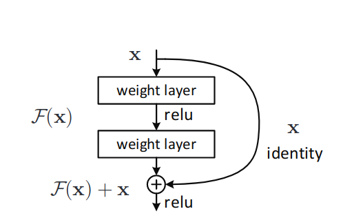
Diagram of a residual connection, from the original paper. The residual connection (right) flows around computational blocks.
Prerequisites#
To follow along with this blog, you will need the following:
Hardware
AMD GPU - see the list of compatible GPUs
OS
Linux - see supported Linux distributions
Software
ROCm - see the installation instructions
Running this blog#
There are two ways to run the code in this blog. First, you can use docker (recommended), or you can build your own python environment (see running on host in the appendix).
Running in Docker#
Using docker is the easiest and most reliable way to construct the required environment.
Ensure you have Docker. If not, see the installation instructions
Ensure you have
amdgpu-dkmsinstalled (which comes with ROCm) on the host to access GPUs from inside docker. See the ROCm docker instructions here.Clone the repo, and
cdinto the blog directorygit clone git@github.com:ROCm/rocm-blogs.git cd rocm-blogs/blogs/artificial-intelligence/resnet
Build and start the container. For details on the build process, see the
dockerfile. This will start a jupyter lab serer.cd docker docker compose build docker compose up
Navigate to http://localhost:8888 in your browser, and open the file
resnet_blog.pyin notebook format (right click -> open with -> notebook)Note
Note: This notebook is a JupyText paired notebook, in py-percent format
Training ResNet 18 on the CIFAR10 dataset#
Below, we will walk through the training code, step by step.
Imports#
First, import required packages
import random
import datetime

import torch
import torchvision
from torchvision.transforms import v2 as transforms
from datasets import load_dataset
import matplotlib.pyplot as plt
Dataset#
For this task, we will use the CIFAR10 dataset, which is available on huggingface. The CIFAR10 dataset consists of 60,000 32x32 images, in 10 classes.
Let’s define a function to retrieve train and test dataloaders. In this function, we (1) download the dataset, (2) set the format to torch, and (3) construct train and test data loaders.
def get_dataloaders(batch_size=256):
    """
    Return test/train dataloaders for the cifar10 dataset
    """
    # Download the dataset, and set format to `torch`
    dataset = load_dataset("cifar10")
    dataset.set_format("torch")

    # Construct train/test loaders
    train_loader = torch.utils.data.DataLoader(dataset["train"], shuffle=True, batch_size=batch_size)
    test_loader = torch.utils.data.DataLoader(dataset["test"], batch_size=batch_size)

    return train_loader, test_loader
Transforms#
The pixels in the images of this dataset are encoded in uint8 format, as such, we need to convert them to float32, and normalize them. The function below constructs a single composed transform to prepare the data for training.
In the function below, we construct a single composed torchvision transform, which does the following:
Permute the channel dimension so that our batch of images is “channel first”, as required by
pytorchConvert to
float32Scale values to be in range [0,1]
Normalize values to be mean 0, std 1
def get_transform():
    """
    Construct and return a  transform chain which will convert the loaded images into the correct format/dtype,
    with normalization
    """
    # The mean/std of the CIFAR10 dataset
    stats = ((0.4914, 0.4822, 0.4465), (0.2023, 0.1994, 0.2010))

    transform = transforms.Compose(
        [
            # This dataset is channels last (B,H,W,C), need to permute to channels first (B,C,H,W)
            transforms.Lambda(lambda x: x.permute(0, 3, 1, 2)),
            # Convert to float
            transforms.ToDtype(torch.float32),
            # Divide out uint8
            transforms.Lambda(lambda x: x / 255),
            # Normalize
            transforms.Normalize(*stats, inplace=True),
        ]
    )
    return transform
Construct model, loss, and optimizer#
Next, we must construct the model, loss function, and optimizer we wish to use during training.
Model: We will use the
torchvisionResNet18, set withnum_classes=10to match the cifar10 dataset.ResNet18is one of the smaller ResNet models (consisting of 18 convolutional layers), and so is suited for a simpler task, such as CIFAR10 classification.Loss function: Cross entropy loss, standard for classification problems
Optimizer: Adam optimizer
def build_model():
    """
    Construct model, loss function, and optimizer
    """
    # ResNet18, with 10 classes
    model = torchvision.models.resnet18(num_classes=10)

    # Standard crossentropy loss
    loss_fn = torch.nn.CrossEntropyLoss()

    # Adam optimizer
    optimizer = torch.optim.Adam(model.parameters(), lr=0.01, weight_decay=1e-4)

    return model, loss_fn, optimizer
Training Loop#
Lastly, we build a simple training loop in PyTorch. Here, we will train the model for a pre-specified number of epochs. During each epoch, we make a complete pass over the train dataset, and compute the training loss. We then make a complete pass over the test dataset, and compute test loss and accuracy.
def train_model(model, loss_fn, optimizer, train_loader, test_loader, transform, num_epochs):
    """
    Perform model training, given the specified number of epochs
    """
    # Declare device to train on
    print(f"Number of GPUs: {torch.cuda.device_count()}")
    print([torch.cuda.get_device_name(i) for i in range(torch.cuda.device_count())])
    device = torch.device("cuda" if torch.cuda.is_available() else "cpu")

    t0 = datetime.datetime.now()
    model.to(device)
    model.train()

    accuracy = []
    # Main training loop
    for epoch in range(num_epochs):
        print(f"Epoch {epoch+1}/{num_epochs}")
        t0_epoch_train = datetime.datetime.now()

        # Iterate over training dataset
        train_losses, n_examples = [], 0
        for batch in train_loader:
            batch = {k: v.to(device) for k, v in batch.items()}

            optimizer.zero_grad()

            preds = model(transform(batch["img"]))

            loss = loss_fn(preds, batch["label"])
            loss.backward()
            optimizer.step()

            train_losses.append(loss)
            n_examples += batch["label"].shape[0]
        train_loss = torch.stack(train_losses).mean().item()
        t_epoch_train = datetime.datetime.now() - t0_epoch_train

        # Perform evaluation
        with torch.no_grad():
            t0_epoch_test = datetime.datetime.now()
            test_losses, n_test_examples, n_test_correct = [], 0, 0
            for batch in test_loader:
                batch = {k: v.to(device) for k, v in batch.items()}

                preds = model(transform(batch["img"]))

                loss = loss_fn(preds, batch["label"])

                test_losses.append(loss)
                n_test_examples += batch["img"].shape[0]
                n_test_correct += (batch["label"] == preds.argmax(axis=1)).sum()

            test_loss = torch.stack(test_losses).mean().item()
            test_accuracy = n_test_correct / n_test_examples
            t_epoch_test = datetime.datetime.now() - t0_epoch_test
            accuracy.append(test_accuracy.cpu())

        # Print metrics
        print(f"  Epoch time: {t_epoch_train+t_epoch_test}")
        print(f"  Examples/second (train): {n_examples/t_epoch_train.total_seconds():0.4g}")
        print(f"  Examples/second (test): {n_test_examples/t_epoch_test.total_seconds():0.4g}")

        print(f"  Train loss: {train_loss:0.4g}")
        print(f"  Test loss: {test_loss:0.4g}")
        print(f"  Test accuracy: {test_accuracy*100:0.4g}%")

    total_time = datetime.datetime.now() - t0
    print(f"Total training time: {total_time}")
    return accuracy
Train the Model#
Finally, we can put it all together in our main method. Here, we:
Set the random seed for reproducibility
Construct all components (model, data loaders, etc)
Call our training method
seed = 0
random.seed(seed)
torch.manual_seed(seed)

model, loss, optimizer = build_model()
train_loader, test_loader = get_dataloaders()
transform = get_transform()

test_accuracy = train_model(model, loss, optimizer, train_loader, test_loader, transform, num_epochs=8)
    Epoch 1/8
      Epoch time: 0:00:15.129099
      Examples/second (train): 3639
      Examples/second (test): 7204
      Train loss: 1.796
      Test loss: 1.409
      Test accuracy: 48.88%
    ...
    Epoch 8/8
      Epoch time: 0:00:07.136725
      Examples/second (train): 8182
      Examples/second (test): 9748
      Train loss: 0.6939
      Test loss: 0.7904
      Test accuracy: 72.87%
    Total training time: 0:00:57.931011
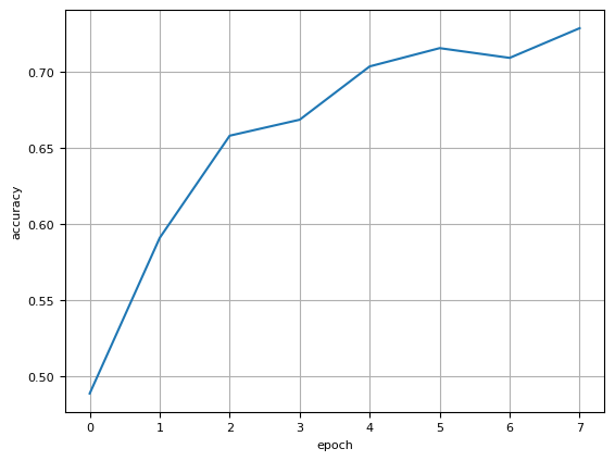
Let’s plot the accuracy over the course of training.
fig,ax = plt.subplots()
ax.plot(test_accuracy)
ax.set_xlabel("epoch")
ax.set_ylabel("accuracy")
plt.show()
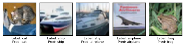
Finally, we can plot some predictions to see how we did.
label_dict = {0: 'airplane',1: 'automobile',2: 'bird',3: 'cat',4: 'deer',5: 'dog',6: 'frog',7: 'horse',8: 'ship',9: 'truck'}

# Plot the first 5 images
N = 5
device='cuda'
for batch in test_loader:
    batch = {k: v.to(device) for k, v in batch.items()}
    preds = model(transform(batch["img"])).argmax(axis=1)
    labels = batch['label'].cpu()

    fig,ax = plt.subplots(1,N,tight_layout=True)
    for i in range(N):
        ax[i].imshow(batch['img'][i].cpu())
        ax[i].set_xticks([])
        ax[i].set_yticks([])
        ax[i].set_xlabel(f"Label: {label_dict[labels[i].item()]}\nPred: {label_dict[preds[i].item()]}")

    break
Summary#
In this blog, we showed how to use AMD GPU to train a ResNet image classifier on the CIFAR10 dataset, achieving 73% accuracy in less than a minute! All of this runs seamlessly on AMD GPUs with ROCm. We can further improve performance by employing several techniques, such as LR schedulers, data augmentation, and more training epochs, which we will leave as an exercise to the reader.
References#
Appendix#
Running on host#
If you don’t want to use docker, you can also run this blog directly on your machine - although it takes a little more work.
Prerequisites:
Install ROCm 5.7.x
Ensure you have python 3.10 installed
Install PDM - used here for creating reproducible python environments
Create the python virtual environment in the root directory of this blog:
pdm syncStart the notebook
pdm run jupyter-lab
Navigate to https://localhost:8888 and run the blog
Disclaimers#
Third-party content is licensed to you directly by the third party that owns the content and is not licensed to you by AMD. ALL LINKED THIRD-PARTY CONTENT IS PROVIDED “AS IS” WITHOUT A WARRANTY OF ANY KIND. USE OF SUCH THIRD-PARTY CONTENT IS DONE AT YOUR SOLE DISCRETION AND UNDER NO CIRCUMSTANCES WILL AMD BE LIABLE TO YOU FOR ANY THIRD-PARTY CONTENT. YOU ASSUME ALL RISK AND ARE SOLELY RESPONSIBLE FOR ANY DAMAGES THAT MAY ARISE FROM YOUR USE OF THIRD-PARTY CONTENT.