Getting Started with AMD AI Workbench: Deploying and Managing AI Workloads#

In this blog, you will learn how to use AMD AI Workbench, an easy to use graphical user interface (GUI) with command-line interface (CLI) support for running and managing AI workloads. It’s part of the AMD Enterprise AI Suite, a full-stack solution for developing, deploying and running AI workloads on a Kubernetes platform designed to support AMD compute. AMD AI Workbench is designed to offer AI developers accelerated end-to-end AI development, from experimentation to production deployment.
The AMD AI Workbench allows you to deploy AMD Inference Microservices (AIMs) from the AIMs catalog. AIMs provide standardized, portable inference microservices for serving AI models on AMD Instinct™ GPUs. AIMs are published and distributed as Docker images on Docker Hub. In addition, you can launch and use development workspaces pre-configured for AMD compute, such as Visual Studio Code (VS Code) or JupyterLab. It is also possible to customize models with your own data, test and compare your models in a chat interface and self-provision GPUs, all in an environment available through both GUI and CLI.
This blog walks you through these capabilities, specifically covering:
How to deploy an AIM and use the AMD AI Workbench interface to interact with it
How to create and access a VS Code workspace within AMD AI Workbench
How to connect to the deployed AIM from the VS Code workspace via the OpenAI-compatible API
Experiment with the deployed AIM and VS Code workspace to test model capabilities
Prerequisites#
This blog utilizes the AMD Enterprise AI Suite. Before proceeding, please ensure the following prerequisites are met:
Access to AMD Enterprise AI Suite: You must have access to an installed instance of the AMD Enterprise AI Suite. Refer to the Supported Environments documentation for installation details.
GPU Resources: You will need a project configured with at least two GPUs. Projects are essential for organizing and isolating resources, workloads, and secrets. For setup assistance, see Manage Projects.
Note: This blog was validated on a node equipped with AMD Instinct™ MI300
Optional: While this blog utilizes a public model, a Hugging Face token is required to explore gated models. Instructions for adding the token to the AMD Enterprise AI Suite are provided later in this blog.
To get the most out of this blog, you should be familiar with:
AMD AI Workbench#
Begin by logging into the AMD Enterprise AI Suite and navigating to the AI Workbench (Figure 1). Before deploying an AIM, review the Workbench components and their capabilities below:
API keys: Manage secure, programmatic credentials for calling deployed models and project resources; support configurable expiration times, renewal, and fine-grained access control by binding them to specific model deployments
Chat: Utilize this interactive interface to query deployed models, adjust generation parameters, test responses in real-time, and compare model outputs
Datasets: Upload and manage datasets on the platform to facilitate fine-tuning
Models: View a comprehensive list of models available for deployment or fine-tuning. This includes the AIM catalog—a collection of production-ready inference services optimized for AMD hardware
Secrets: Secure storage for sensitive values (e.g., Hugging Face tokens, API credentials, storages)
Workloads: Monitor all active workloads (batch jobs or services running in the cluster) and access detailed execution statistics
Workspaces: Access various web-based, zero configuration interactive environments such as VS Code and MLflow
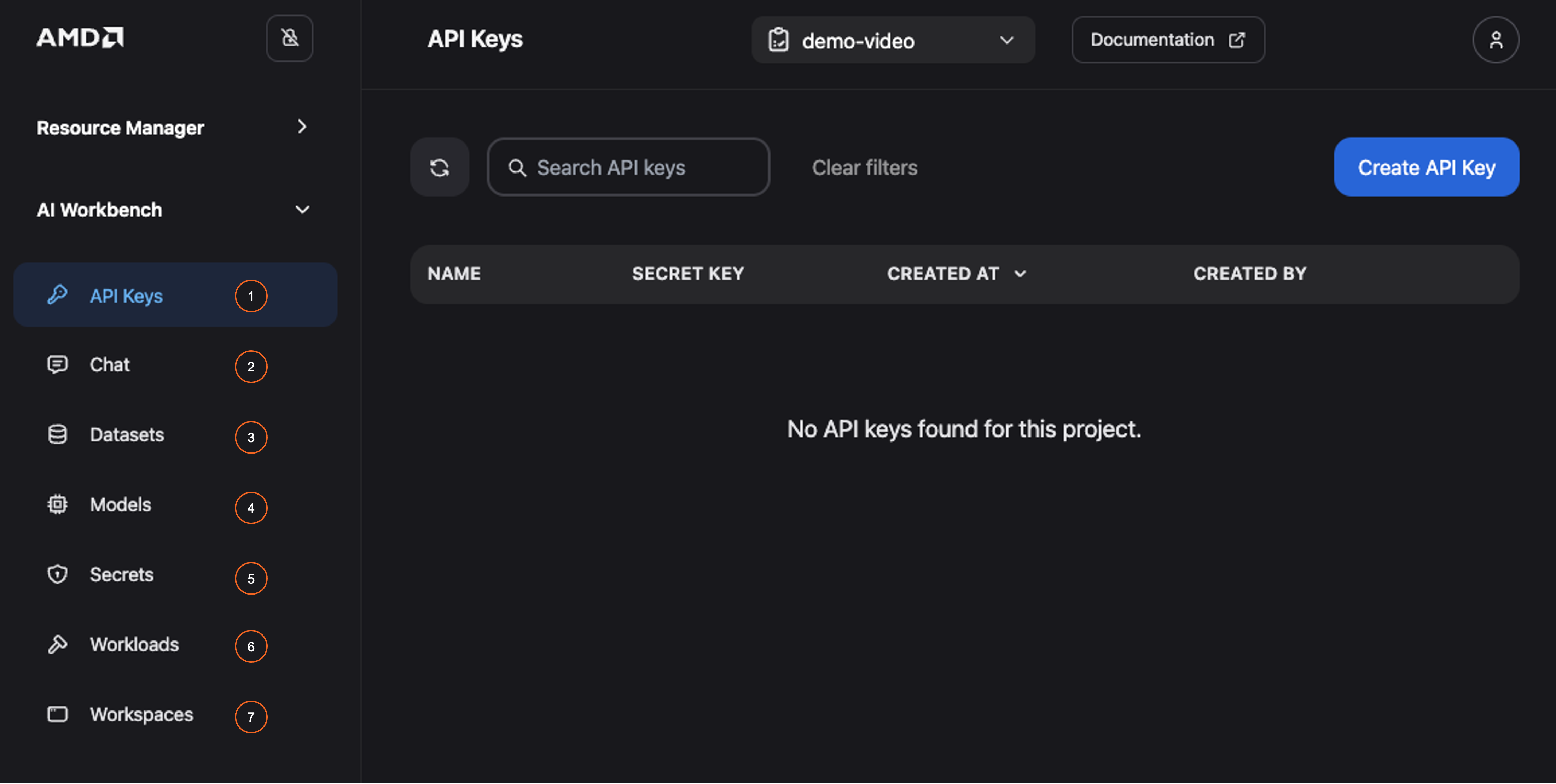
Figure 1: Overview of AMD AI Workbench.
Deploy an AMD Inference Microservice (AIM)#
With the AI Workbench overview complete, we can now demonstrate the streamlined process for deploying an optimized inference service. This example will guide you through deploying an AIM directly from the Models page within the AI Workbench.
Note
AIMs also support deployment via Kubernetes, KServe, or Docker. Please refer to the technical documentation for further details.
Deployment#
Navigate to the Models tab. Here, you will find the AIM catalog, a curated collection of open-source models from the Hugging Face community. From this page, you can download and deploy models you want to use.
AIMs provide standardized, production-ready services for state-of-the-art large language models (LLMs). Each AIM container comes with built-in model caching and hardware-aware optimizations for AMD Instinct GPUs.
In this blog, we’ll download the mistralai/Mistral-Small-3.2-24B-Instruct-2506 model:
Go to the model card and click on the three dots in the bottom right corner (See Figure 2)
Select Deploy
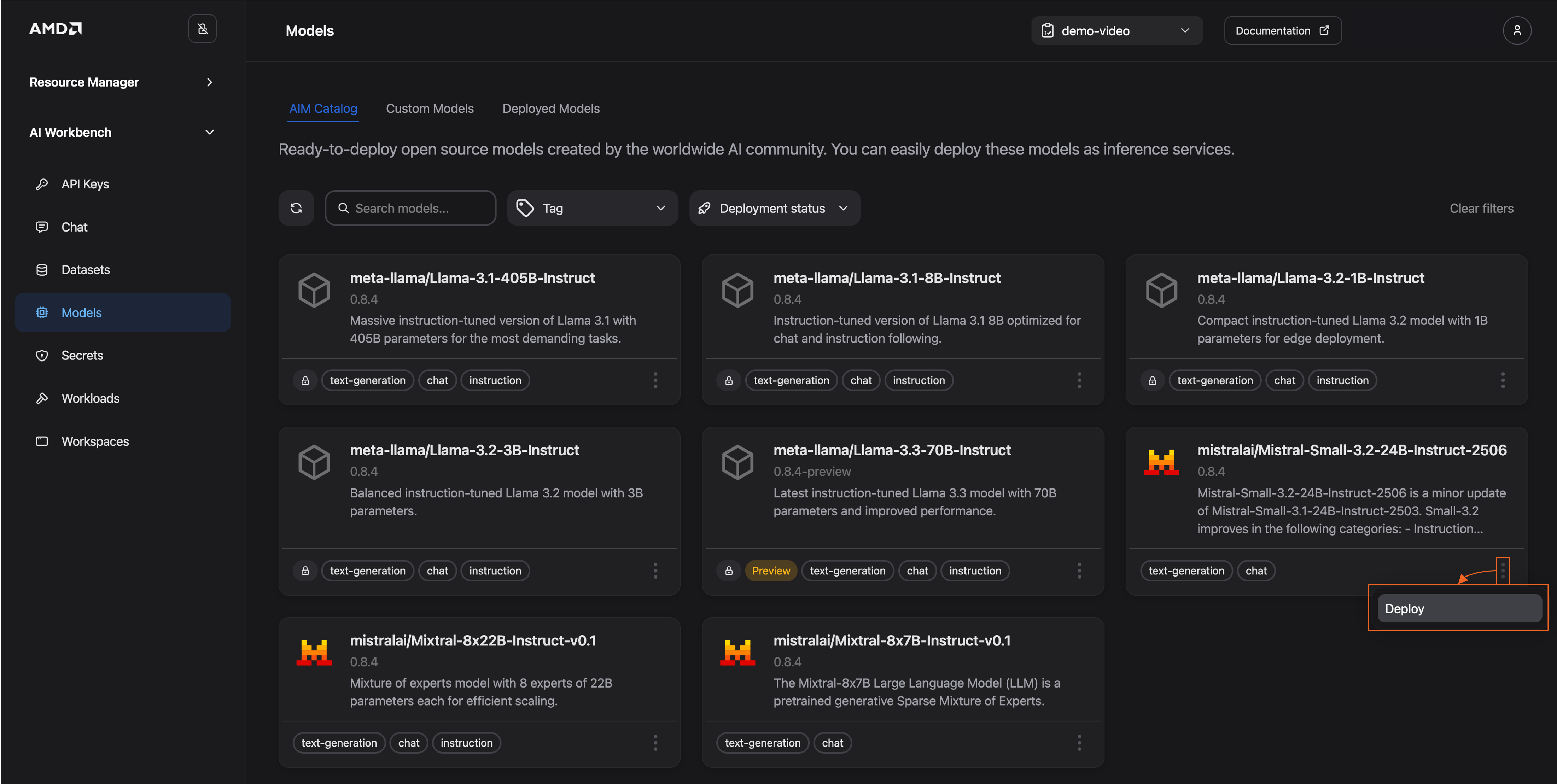
Figure 2: Open deployment settings.
Choose your desired configuration (See Figure 3). For this blog, select Default, which automatically picks the most appropriate metric based on your model and hardware. You may also manually choose between:
Latency: Prioritize low end-to-end latency; or,
Throughput: Prioritize sustained requests/second
You can also allow for “Unoptimized deployment”
This option allows deployment of the AIM to hardware it is not specifically optimized for
Deploy the workload
You will receive confirmation that the workload has started
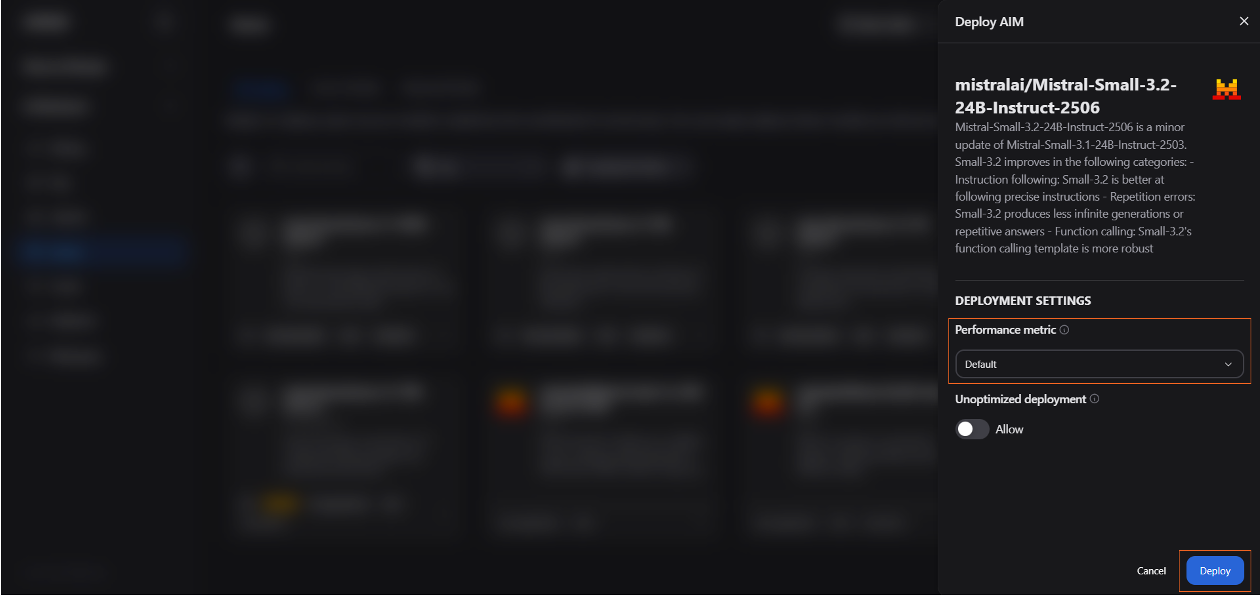
Figure 3: Select a configuration and deploy
The model used in this example is public and does not require a Hugging Face token. However, if you wish to deploy a gated model (such as those from the Llama family), which is indicated by a lock icon on its model card, you must provide a Hugging Face token for access. Adding a token is straightforward:
Choose your gated model and click Deploy to enter deployment settings as before
In the deployment menu, you will be prompted for a token (See Figure 4). You can either:
Select a pre-existing token or;
Add a token directly
Once the token is selected or added, click Deploy to start the workload
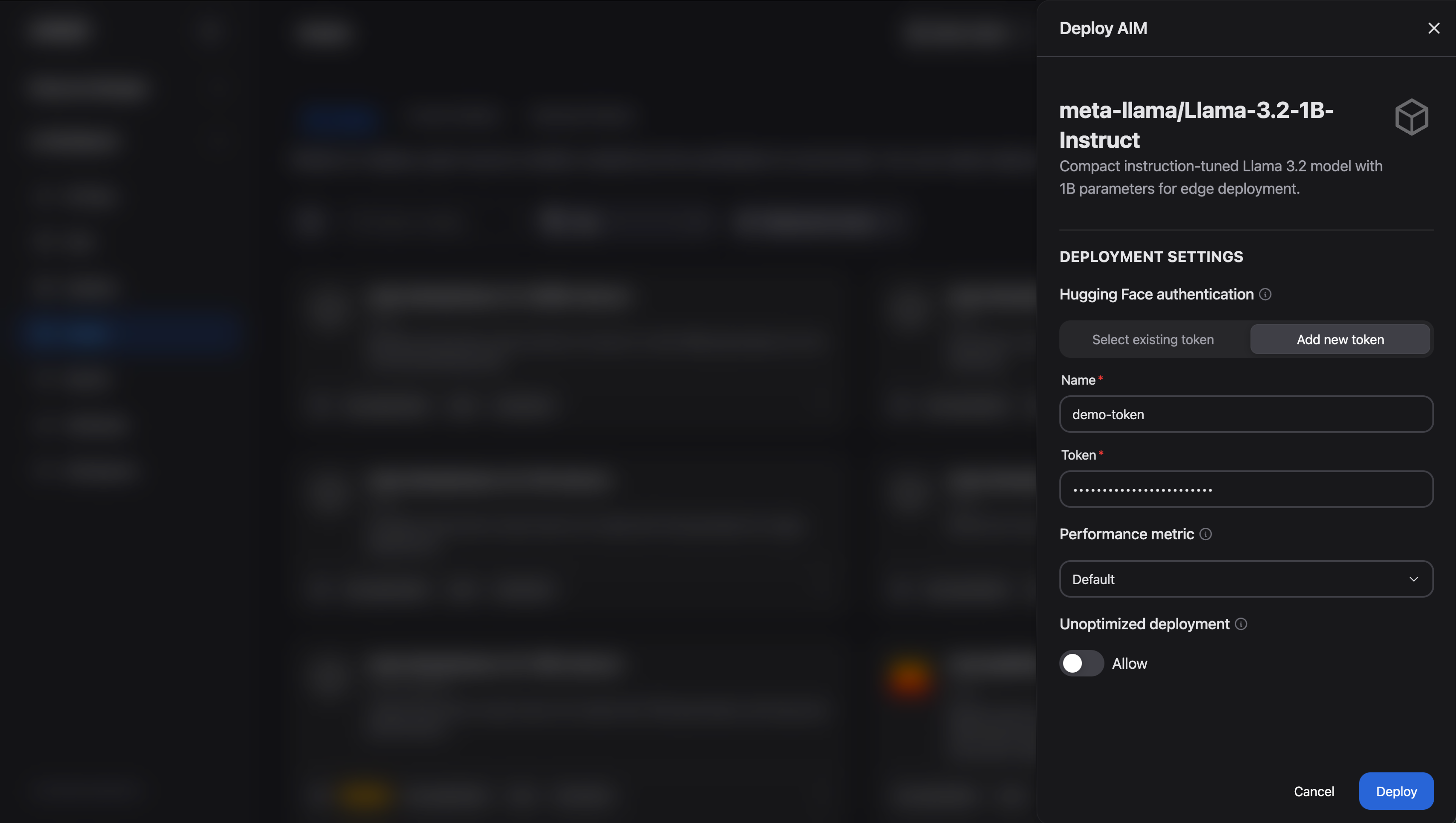
Figure 4: Add a Hugging Face token.
Monitor the deployment#
While the model downloads and initializes, you can monitor its deployment status:
Navigate to either the Deployed Models tab (on the Models page) or the Workloads page
Observe the status of your new workload
Wait for the status to transition from Pending to Running
Interact with the model#
Once your model is successfully deployed, you can interact with it in two primary ways:
Chat Interface: Use the built-in Chat page within the AI Workbench for direct interactive testing
API Integration: Programmatically access the model using the AIM’s OpenAI‑compatible API endpoint
Chat via the Workbench interface#
We’ll begin by using the Chat interface. The Chat page is ideal for exploratory testing, prompt engineering, and receiving immediate feedback from your deployed models.
To interact with your model, follow these steps:
Navigate to the Deployed Models tab, pick your model and click Chat with model, or open the Chat page directly from the main navigation menu and then select your model
Enter your prompt in the chat box and submit it to the model
Experiment with the model’s output by adjusting generation parameters (see Figure 5 below). Access these controls, such as
temperature, by clicking the settings toggle in the upper-right corner.Review the response in the chat window and refine your prompt or parameters as needed to achieve the desired result
For example, you can submit a simple prompt like, “What is the capital of Sweden?” and then observe how modifying the generation parameters affects the detail and style of the answer.
Output:
The capital of Sweden is Stockholm. It is located on the eastern coast of Sweden, where Lake Mälaren meets the Baltic Sea. Stockholm is known for its beautiful archipelago, historic sites like the Royal Palace, and vibrant cultural scene. It is also the largest city in Sweden.
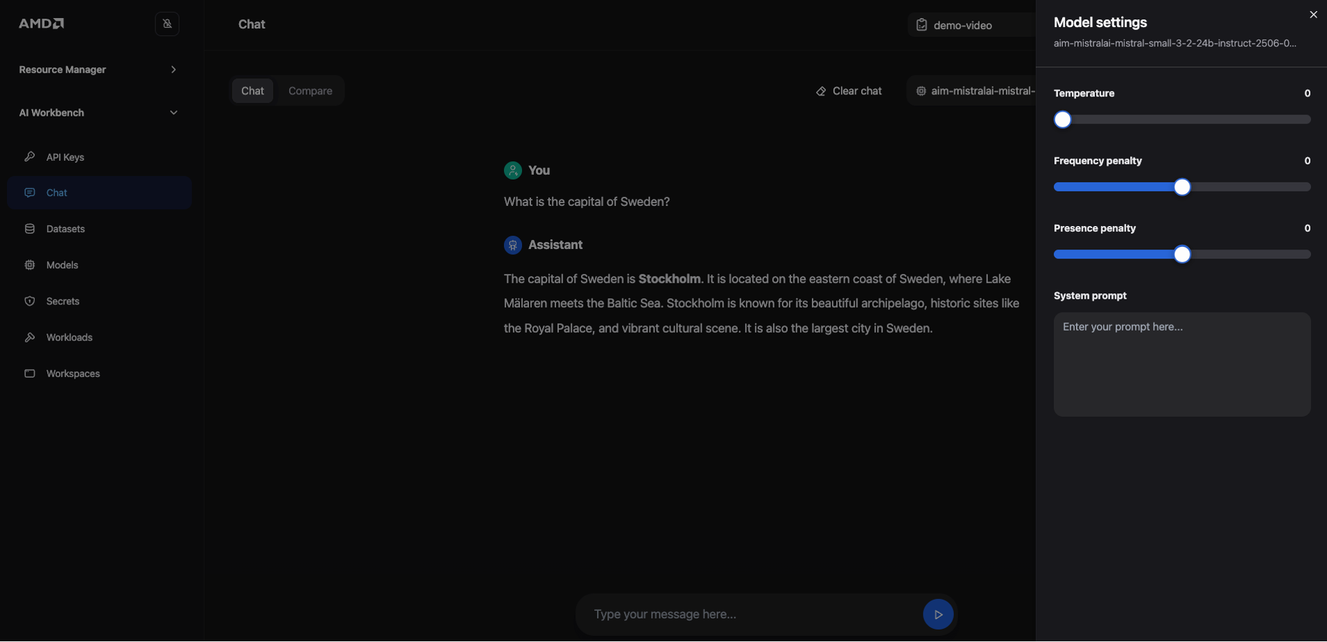
Figure 5: Chat with the model directly in the Workbench interface.
The Chat interface also includes a Compare mode. This feature sends the same prompt to two models (or the same model with different settings) and displays their responses side‑by‑side, making it easy to evaluate differences in responses, accuracy, tone, and reasoning. Typical use cases include comparing a base model against its fine-tuned version or testing how different system prompts and generation parameters affect a single model’s behavior.
Let’s demonstrate this feature by comparing our deployed model against itself, but with a modified system prompt:
Click the Compare toggle at the top of the Chat page to activate the dual-panel view
In the selection box (“Select model”), choose your deployed model
For the model on the right, open its settings panel and change the System Prompt to the following:
“You are a helpful AI model that always provides happy and cheerful answers.”
Enter the prompt “What is the capital of Sweden?” and submit it
Observe how the two models provide different responses with one delivering a standard factual answer and the other adopting a cheerful persona (See Figure 6)
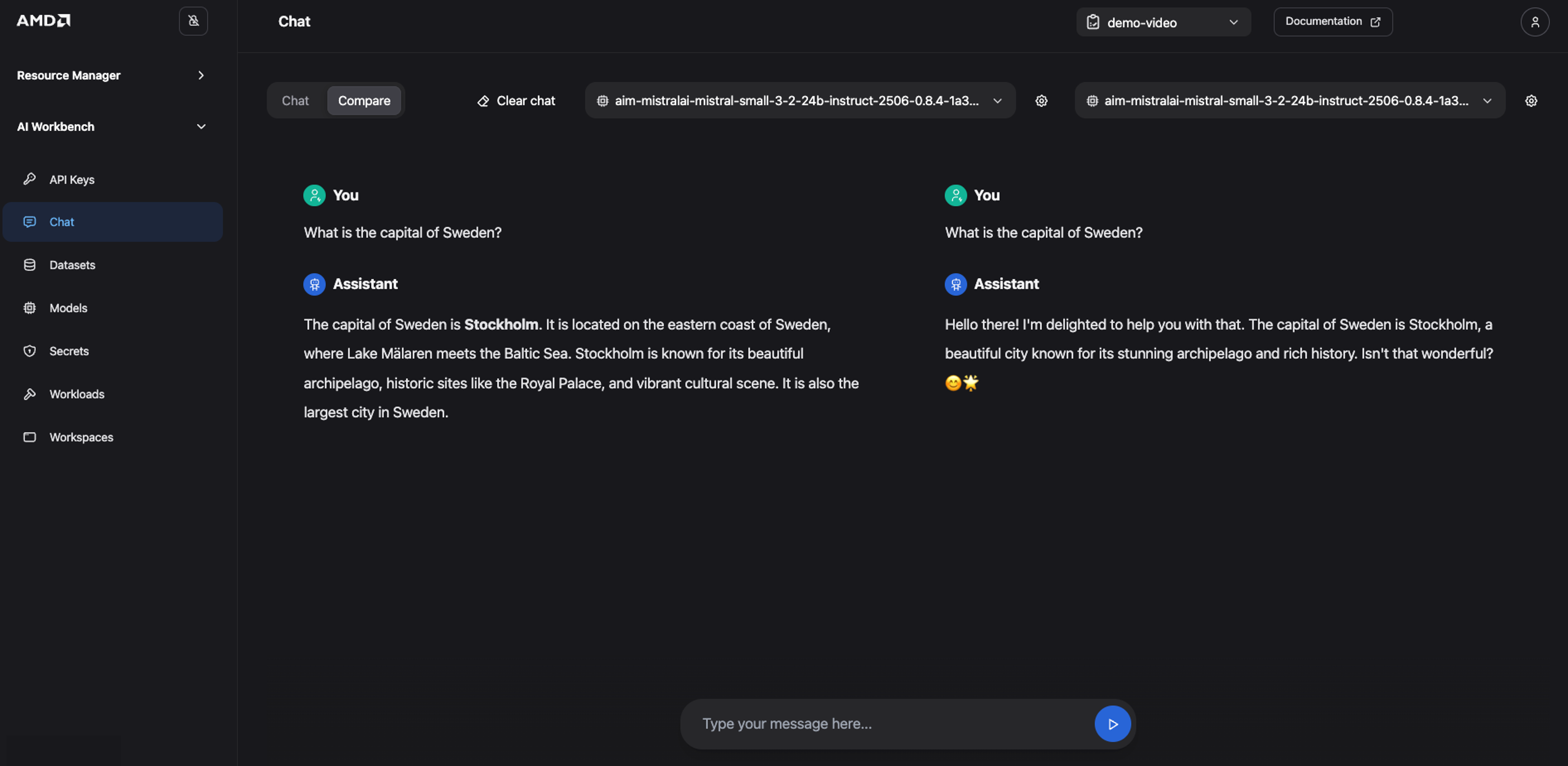
Figure 6: Compare model output.
Use the AIM’s OpenAI‑compatible API#
For advanced users, AIMs provide an OpenAI-compatible API for LLMs, making integration with your applications easier. To demonstrate this capability, we will launch a VS Code workspace from the Workspace page inside the AI Workbench.
Note
Using a Workspace is just one convenient method for API interaction. You do NOT need to use a Workspace to connect to the model. You can connect to a deployed model’s endpoint both internally (AMD Enterprise AI Suite) and externally, including your local machine. Instructions for generating the necessary credentials and connection details for both internal and external access will be provided shortly.
Create and access a Visual Studio Code workspace#
From the Workspace page, you can launch pre-configured development workspaces to accelerate experimentation. For example, JupyterLab and VS Code workspaces enable users to harness the power of the cluster with zero configuration on their local machines.
Deploy your VS Code workspace#
Navigate to the Workspaces page, where you will find a catalog of available workspaces:
Locate the VS Code card and click View and deploy. This will open the deployment configuration view where you can customize your workspace before deployment (See Figure 7).
Configure the following settings:
Workload name: Give your workspace a unique name
Container image: Keep the default image. The workspace will automatically pull and run the image upon deployment.
Customize resource allocation: Allocate hardware resources using the provided sliders. The following configuration was used to validate this blog:
GPU: 1
CPU: 8 cores
RAM: 32 GB
Once you have finalized the configuration, launch the environment by clicking Quick deploy
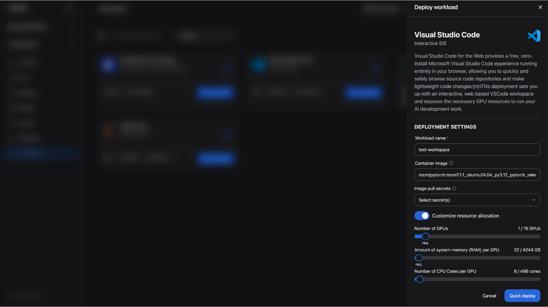
Figure 7: Deploy a Visual Studio Code workspace.
As with AIM deployments, you can monitor the status of your workspace on the Workloads page. It will show Pending while the resources are being provisioned.
Launch the workspace#
Once the workspace is ready, the deployment overlay will display a Launch button (See Figure 8). Click it to open your workspace.
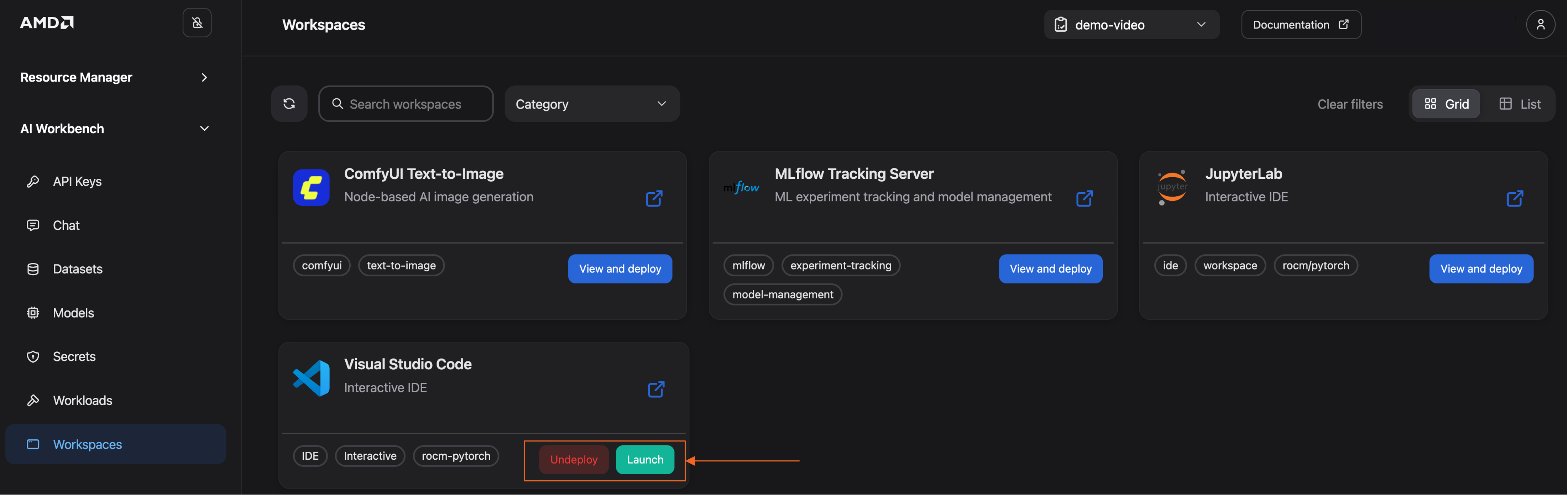
Figure 8: Launch the Visual Studio Code workspace.
Inside the VS Code workspace, you can operate as you would in a regular VS Code project. For example, you can open a terminal, create / upload and run your files. Note that a persistent storage volume is automatically mounted at the top level of the workload directory, ensuring your files are preserved across sessions.
For the next steps, you will need to create a Jupyter Notebook:
Click New file from the File menu
Choose the Jupyter notebook file type or create a new file and save it with the file extension “.ipynb”
If you want to save it, make sure it’s saved in your persistent storage directory
From this point forward, all code provided in this blog should be executed within this notebook.
Connect to the model from the workspace via the OpenAI-compatible API#
Retrieve connection details#
To connect to your deployed model, you first need to retrieve its unique API endpoint:
Navigate to the Models page
Select the deployed model (same button we used to deploy the model)
Click the Connect button
This will open a dialog window displaying the essential connection details, specifically the External URL (for connections outside the platform) and the Internal URL (for connections inside the platform, such as a workspace). See Figure 9 for reference.
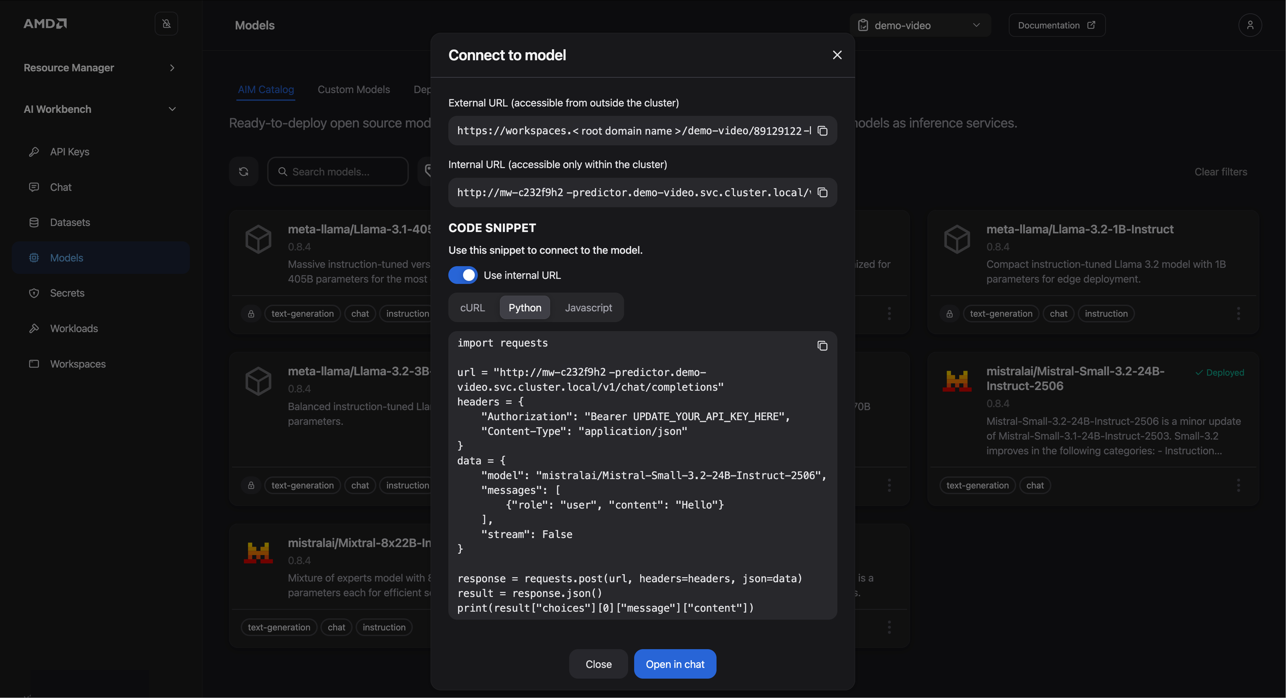
Figure 9: Connection details.
The window also provides sample code for querying the model in cURL, Python and Javascript format. We will use the Python snippet to connect from our VS Code notebook:
Since our notebook is running inside the platform, select the Internal URL
Choose the Python tab to view the corresponding Python code snippet
Click the Copy icon in the top-right corner and paste the code into a new cell in your Jupyter notebook
Finally, modify the sample code to send a more specific prompt. Locate the line that defines the user message and update it as shown below:
“content”: “Hello!”to“content”: “What is the capital of Sweden?”
The request should look like this:
import requests

url = "YOUR_INTERNAL_URL"
headers = {
    "Authorization": "Bearer UPDATE_YOUR_API_KEY_HERE",
    "Content-Type": "application/json"
}
data = {
    "model": "mistralai/Mistral-Small-3.2-24B-Instruct-2506",
    "messages": [
        {"role": "user", "content": "What is the capital of Sweden?"}
    ],
    "stream": False
}

response = requests.post(url, headers=headers, json=data)
result = response.json()
print(result["choices"][0]["message"]["content"])
Note
If you want to test the model manually before coding, you can click the “Open in chat” button to jump directly to the Chat interface we used before.
Run your request#
Since we are using an internal connection, an API key is not required for authentication. You can now execute the code cell containing the Python script. Depending on the container image, you might need to install the requests library before running the code:
!pip install requests
When you run the notebook for the first time, you may be prompted to select a kernel for your notebook. If prompted, install or choose the appropriate Python environment. Once the kernel is active, the notebook will execute the code and display the results.
If the connection is successful, you should receive an answer like the one below. The exact phrasing may vary slightly with each execution, which is expected behavior for large language models:
The capital of Sweden is Stockholm. It is located on the eastern coast of the country, where Lake Mälaren meets the Baltic Sea. Stockholm is known for its beautiful archipelago, historic sites like the Royal Palace, and vibrant culture.
Generate an API key#
To connect to your model from an external application, such as one running on your local machine, you must first generate an API key to authenticate your requests.
Creating an API key is straightforward:
Navigate to the API Keys page in the Workbench
Click on Create API Key
Fill in the required information and ensure you assign the key to the deployed model
Click Create API key
Copy the generated API key and replace the placeholder
“UPDATE_YOUR_API_KEY_HERE”with this key (Python code snippet)
Finally, remember to update the URL in your code to point to the External URL.
Note
Important: Copy and save your API key in a secure location immediately. For security reasons, the key will only be visible once upon creation.
Monitor inference endpoint#
In this example, we are connecting to the model to verify the setup; however, if this workload was running in production—serving one or multiple products—monitoring the inference endpoint logs and metrics would be essential for maintaining reliability, detecting regressions, and planning capacity.
To monitor your inference endpoint, open the Workloads page, select the workload (use the three dots on the far right) and choose “Open details” (See Figure 10 below).
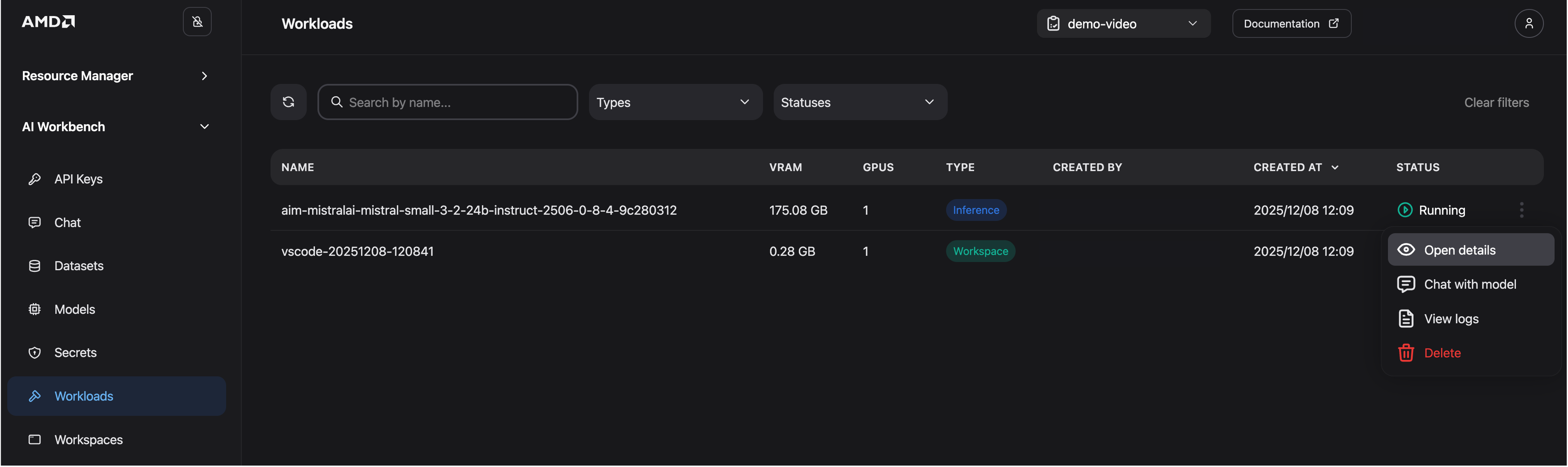
Figure 10: Open for more details.
The details’ view lets you inspect and review inference metrics over time such as time‑to‑first‑token, request count, tokens generated and other indicators (Figure 11). It also shows workload metadata such as resource utilization, AIM build/version, and configuration settings.
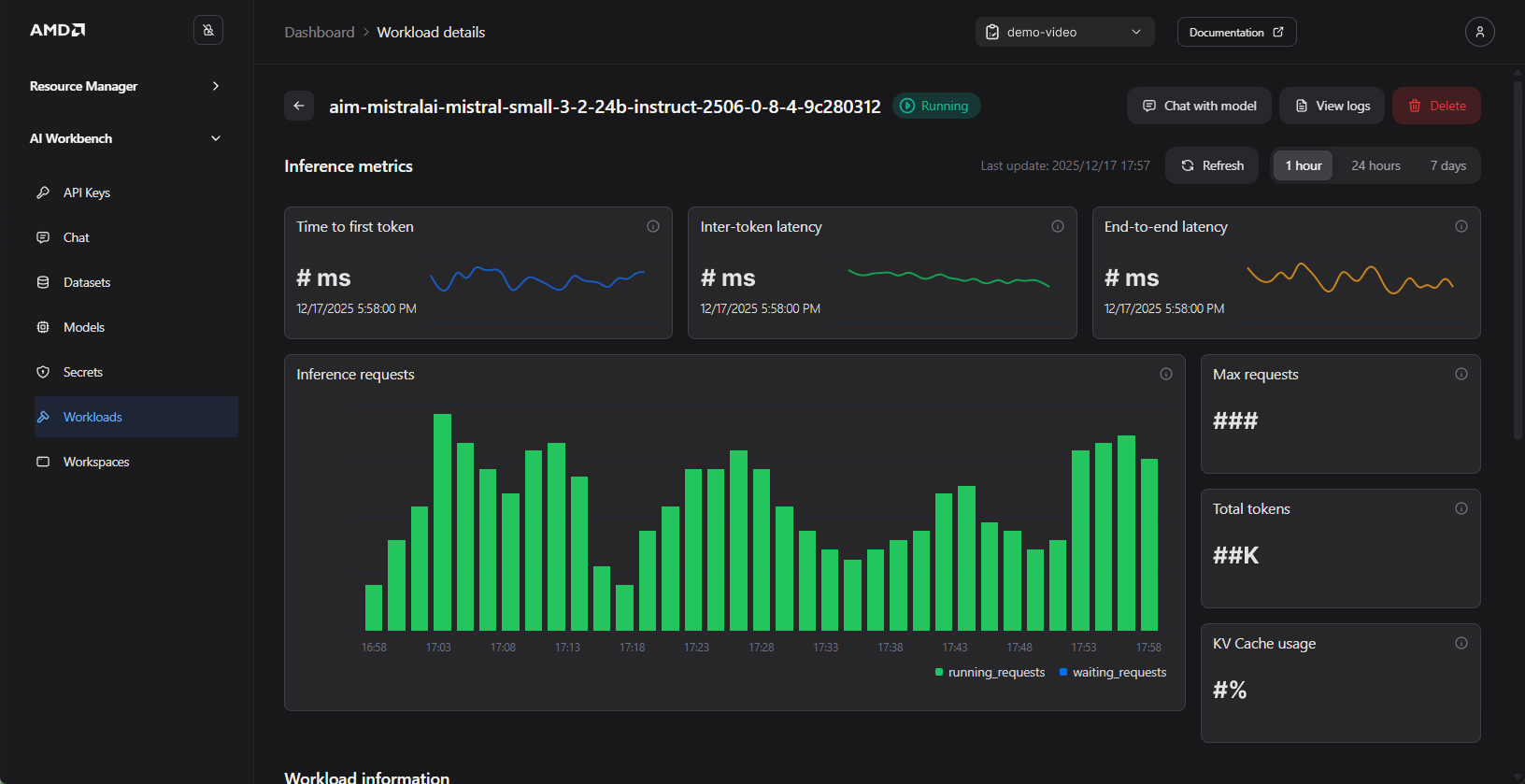
Figure 11: Monitor the status of your workload. For illustration purposes only.
Experimentation within the workspace#
Now that you’ve successfully connected to the model, it’s time to experiment and explore practical use cases. You might want to:
Integrate the model into your custom applications
Benchmark the model’s performance on specific tasks
Build an agent
Implement a Retrieval-Augmented Generation (RAG) pipeline
Apply the model to your own data for tasks like sentiment analysis, summarization, or classification
To demonstrate how you can experiment with your deployed models within the workspace, we will implement a simple RAG pipeline using ChromaDB. The goal is to enable the model to answer questions about custom data, in this case fictional products that were not part of its original training set.
Please continue to use the same VS Code notebook as before.
RAG#
A general RAG pipeline consists of four steps:
Submit – The user sends a query to the system
Retrieve – A vector store retrieves relevant chunks of information (context) based on the query
Augment – The retrieved context is combined with the query to form a new, more detailed prompt
Generate – The model uses the augmented prompt to produce a context-aware answer
We will now walk through a simplified implementation of these steps without detailed explanations. If you are keen to learn more about RAG, it’s highly recommended to check out our previous blogs:
Dependencies#
First, install the required dependencies inside your notebook:
!pip install chromadb
Next, import the necessary libraries.
import requests
import chromadb
Submit a query#
We will now create a reusable function to query our deployed model. This function will build upon the code from the previous section but will also incorporate a system prompt to guide the model’s behavior:
def query_model(system_prompt, user_query):
    """
    Query the model using the provided user question and system prompt.
    """

    url = "YOUR_INTERNAL_URL"
    headers = {
        "Authorization": "Bearer UPDATE_YOUR_API_KEY_HERE",
        "Content-Type": "application/json"
    }
    data = {
        "model": "mistralai/Mistral-Small-3.2-24B-Instruct-2506",
        "messages": [
            {"role": "user", "content": user_query},
            {"role": "system", "content": system_prompt}  # new system prompt
        ],
        "stream": False
    }

    response = requests.post(url, headers=headers, json=data)
    result = response.json()

    return result["choices"][0]["message"]["content"]
Now, let’s test the function by querying the model about a fictional product with ID 456. This will help demonstrate how the model responds when queried about topics or facts it has not encountered before, which is a crucial first step in understanding the need for RAG.
Execute the following code to test the function:
# Prepare the system and user prompts
system_prompt = "You are a helpful assistant. Answer the user's question. If you don't know the answer, say you don't know."
user_query = "What are the 2024 sales numbers for Product ID 456?"

# Execute the query and print the result
query_model(system_prompt, user_query)
As expected, the model correctly identifies that it does not have access to this information and avoids inventing an answer (a behavior known as “hallucination”). The response should be similar to the following:
I don’t have access to real-time sales data or specific databases, so I can’t provide the 2024 sales numbers for Product ID 456. To get this information, you might need to check your company’s internal sales reports, inventory management system, or contact the relevant department (e.g., sales, finance, or operations). If you have access to a CRM or ERP system, you could also look it up there.
Create a vector database#
To enable the model to answer questions about our fictional products, we must provide it with the relevant information. This is accomplished by augmenting the prompt with context retrieved from a knowledge base. For this purpose, we will store our fictional product data in a vector database using Chroma (an open‑source AI application database). The process is as follows:
Each text document is converted into a vector representation using an embedding model
When a user query is made, the system compares the query vector to the vectors in the database using a similarity measure, such as cosine similarity, to identify relevant information
The extracted context is then provided to the language model along with the original query, enabling it to generate a context-aware response
Let’s create the Chroma database. By setting chroma_data_path to a local directory, Chroma will persist its data there. After executing the code below, a new chroma_db_storage folder will be created in your workspace’s persistent storage (or in the folder where your notebook is saved):
chroma_data_path = "chroma_db_storage" # Local path for ChromaDB
collection_name = "simple_rag"

client = chromadb.PersistentClient(path=chroma_data_path)
collection = client.get_or_create_collection(name=collection_name)

print(f"ChromaDB client initialized. Collection '{collection_name}' ready.")
print(f"Items in collection: {collection.count()}")
ChromaDB client initialized. Collection 'simple_rag' ready.
Items in collection: 0
Add example documents to chroma#
Now, let’s populate our vector database with some sample data. In a real-world application, you would typically source and chunk content from your organization’s knowledge bases, such as internal documents or other repositories. However, since this is a simple example, we will use a few simple text strings representing product information.
Add the following documents to your Chroma by running this code in a new cell:
# Add three dummy chunks to the existing ChromaDB collection
docs = [
"Product ID 123 - Sales numbers 2024: SEK 300m",
"Product ID 456 - Sales numbers 2024: SEK 503m",
"Product ID 789 - Sales numbers 2024: SEK 102m",
]

collection.add(
ids=["prod-123", "prod-456", "prod-789"],
documents=docs
)

print(f"Items in collection after insert: {collection.count()}")
Items in collection after insert: 3
The next step in our RAG pipeline is to retrieve relevant information based on a user’s query. This step uses semantic search to find the chunks that are most closely related to your question. These chunks are then added to the prompt. The helper function below encapsulates this retrieval logic, querying the ChromaDB collection and returning the most relevant document:
def query_chroma(prompt, n_results=1):
    """
    Query the ChromaDB collection and return the top n_results documents
    joined into a single context string.
    """
    results = collection.query(
        query_texts=[prompt],
        n_results=n_results,
        include=["documents"],
    )

    retrieved_docs_text = []
    docs = results.get("documents", [[]])[0] if isinstance(results, dict) else []
    for i, doc_text in enumerate(docs):
        retrieved_docs_text.append(doc_text)

    return "\n\n".join(retrieved_docs_text)
Let’s test our retrieval function with a sample query to see it in action:
query_chroma("Sales figures for product 456")
The function should successfully find and return the relevant document from our database:
Product ID 456 - Sales numbers 2024: SEK 503m
Feel free to experiment by adding more documents to your collection or by trying different queries to see how the retrieval works.
Augment and generate#
We will now combine the retrieval and generation steps to complete our RAG pipeline. The following function orchestrates this process by first querying the vector database for relevant context and then using that context to build an augmented prompt.
Notice that the system prompt is updated to explicitly instruct the model to use the provided context when formulating its answer.
def augment_and_generate(user_question, n_results=1):
    """
    Retrieve context from ChromaDB, build a system prompt containing that context,
    and query the model with the augmented prompt.
    """
    # 1) Retrieve context from ChromaDB
    context = query_chroma(user_question, n_results=n_results)

    # 2) Build a system prompt with the retrieved context
    system_prompt = (
        "You are a helpful assistant. Use the provided context to answer the user's question."
        "If the answer is not in the context, say you don't know.\n\n"
        f"Context:\n{context if context else '[No relevant context retrieved]'}"
    )

    # 3) Query the model with the augmented prompt
    return query_model(system_prompt=system_prompt, user_query=user_question)
Let’s ask the same question as before. This time, our augment_and_generate function will automatically retrieve the necessary context before querying the model:
answer = augment_and_generate("What are the 2024 sales numbers for Product ID 456?", n_results=1)
print("Model answer:\n", answer)
The answer is now accurate, as the model has received the domain specific information that it was not trained on:
Model answer:
The 2024 sales numbers for Product ID 456 are SEK 503 million
Summary#
In this blog, we demonstrated the practical steps for deploying and managing AI workloads using AMD AI Workbench. We began by deploying an AMD Inference Microservice (AIM) for optimized inference, verifying its functionality directly through the Chat UI. Following this, we deployed a workspace to facilitate hands-on experimentation with the AIM inference endpoint within the platform.
Now that you’ve seen how AMD AI Workbench simplifies managing your AI inference deployments, you’re ready to deploy your preferred model, create API keys, and integrate it seamlessly into your applications. Start exploring and bring your AI projects to life!
Get started#
AMD AI Workbench is part of the broader AMD Enterprise AI Suite, which provides unified components for scalable inference, resource management, and practitioner tooling. For a greater understanding of the AMD Enterprise AI Suite, see the previous blog post.
Ready to build on what you have learned? Use the resources below to start your journey with the AMD Enterprise AI Suite.
For an overview of the AMD Enterprise AI Suite and AIM:
Visit the AMD Enterprise AI Suite product page
Visit the AMD Enterprise AI Suite developer page
Visit the AMD Inference Microservice (AIM): Production Ready Inference on AMD Instinct™ GPUs blog post
Additional technical documentation from installation to AIM deployment is readily available:
If you are interested in fine-tuning, see the following:
Disclaimers#
Third-party content is licensed to you directly by the third party that owns the content and is not licensed to you by AMD. ALL LINKED THIRD-PARTY CONTENT IS PROVIDED “AS IS” WITHOUT A WARRANTY OF ANY KIND. USE OF SUCH THIRD-PARTY CONTENT IS DONE AT YOUR SOLE DISCRETION AND UNDER NO CIRCUMSTANCES WILL AMD BE LIABLE TO YOU FOR ANY THIRD-PARTY CONTENT. YOU ASSUME ALL RISK AND ARE SOLELY RESPONSIBLE FOR ANY DAMAGES THAT MAY ARISE FROM YOUR USE OF THIRD-PARTY CONTENT.