Performance Profiling on AMD GPUs - Part 7: AI/PyTorch® Edition

November 04, 2026 by Asitav Mishra, Sidafa Conde, Kumar Saurabh, Gina Sitaraman, Vijayalaxmi Pujar.

23 min read. | 5602 total words.

Software tools & optimizations

AI/ML, HPC, Profiling, Performance, PyTorch, Optimization

HPC

This blog, like the previous articles in the profiling guide series (Part 1, Part 2, Part 3, Part 4, Part 5, and Part 6), applies a systematic profiling workflow to a GPU-accelerated application. Those posts establish the core loop on HIP and Fortran applications: baseline timing, kernel hotspots with rocprofv3, rooflines and hardware counters with rocprof-compute, and whole-system timelines with rocprof-sys. Here we apply that loop to a PyTorch training workload, where one logical operator can lower to many GPU kernels and optimization often means changing how the framework dispatches work rather than rewriting a kernel.

AI vs HPC note: The profiling loop is unchanged, but one distinction from HPC drives everything that follows. An HPC application is compiled ahead of execution, a PyTorch workload compiles during it. With torch.compile, kernels are traced and generated on the first iteration, and Triton kernels are just-in-time (JIT) compiled and auto-tuned the first time each tensor shape is seen; even in eager mode the first step pays one-time warm-up costs (HIP context, rocBLAS/MIOpen init, Triton JIT). Separate warm-up from measurement and read timing and counters from steady-state steps only; otherwise the profile reflects the compiler, not the model.

1. What you already know:

   • You run GPU-accelerated PyTorch code (training or stepping a model forward) and can match CLI knobs such as batch size, sequence length, and step count across runs.

   • You understand that one logical operator (for example, attention or a layer norm) can map to many GPU kernels, and that fusion or custom kernels change kernel counts and kernel names.

   • You recognize that a training step has both a forward and a backward pass, and that the backward pass is often the larger of the two.

   • Optional: you have compared runtime across hardware vendors and want AMD-specific traces and counters to explain the gap.

2. What this guide will teach you:

   • Annotate from Python with ROCTx markers via torch.cuda.nvtx (the namespace is CUDA-named, but torch.cuda is PyTorch’s device API on a ROCm™ build as well, and ROCTx mirrors the NVTX range calls, so the same annotations serve either runtime), then trim the timeline with --selected-regions so it maps onto the model and stays readable.

   • Analyze hardware counters with rocprof-compute, using iteration multiplexing to collect the full counter set in a single pass.

   • Evaluate three optimizations (PyTorch-level fusion, torch.compile, and custom Triton kernels) and learn to tell a real win (fusion) from a change that only pays off under the compiler (Triton) by comparing kernel counts, timelines, and throughput.

Profiling Basics

The workflow set out below is the one we apply to optimize ROCm-based PyTorch workloads. We establish a baseline, capture a whole-run system trace with rocprof-sys-run, annotate it with ROCTx and narrow it with rocprof-sys --selected-regions, summarize kernels with rocprofv3, and analyze bottlenecks with rocprof-compute using its iteration-multiplexing option. Each optimization is then measured against that baseline using the same set of tools. The rest of the post walks through this loop on the TinyOpenFold example.

The TinyOpenFold Example

OpenFold is a trainable reproduction of AlphaFold 2. Its performance-critical core is the Evoformer, a stack of blocks that each refine two tensors: a multiple sequence alignment (MSA) representation (B × N_seq × N_res × d_msa) and a pair representation (B × N_res × N_res × d_pair). Each block mixes the two, then refines the pair tensor with the triangle operations that give the pattern its name, a triangular multiplicative update and a triangular self-attention, both of which update every residue pair (i, j) by routing information through a third residue k. TinyOpenFold shrinks this stack (fewer blocks, smaller channel widths, synthetic batches) while keeping that pair/triangle pattern intact, so training runs are short. The defaults are d_msa = 64, d_pair = 128, and n_blocks = 4, which together give approximately 2.64M parameters. For the full block-by-block breakdown, see the upstream ARCHITECTURE.md.

For profiling, two properties of the pair tensor matter most: it is quadratic in sequence length, so it drives O(N_res²) activation memory, and the triangle stages that update it (multiplication and self-attention) drive O(N_res³) compute, N_res² pairs each reduced over all N_res choices of k. Those triangle stages are the dominant compute at moderate N_res and the first place to look in any trace. In addition to that intrinsic cost, the readable baseline pays for many small kernel launches and tail elementwise kernels, the launch-bound fragmentation that fusion (version 2) removes. The profiler separates the math-bound triangles from that launch-bound overhead.

TinyOpenFold ships three implementations of the same model. When comparing performance between implementations, use the same training knob values.

Stage	Directory	Entry point	Role
Version 1	version1_pytorch_baseline/	tiny_openfold_v1.py	Baseline: clean, readable PyTorch. Many kernels per step, the reference for hotspots and operator-to-kernel mapping.
Version 2	version2_pytorch_fused/	tiny_openfold_v2.py	PyTorch fusion: query, key, and value (QKV) and triangle projections fused; fewer dispatches, lower peak memory.
Version 3	version3_triton/	tiny_openfold_v3.py	Triton kernels: custom fused LayerNorm plus fused scaled dot-product attention (SDPA) and QKV fusion, wrapped in autograd functions.

Getting the Code

Clone the canonical repository and enter the example directory:

git clone https://github.com/amd/HPCTrainingExamples.git
cd HPCTrainingExamples/MLExamples/TinyOpenFold

The project README documents the quick start and scaling helpers, and ARCHITECTURE.md walks through the parameter math block by block.

Environment Setup (ROCm + PyTorch)

We validated this post on ROCm 7.13 with PyTorch 2.11 and Triton 3.6 on an AMD Instinct™ MI300X. There are two ways to obtain this stack, depending on whether the ROCm runtime comes from the Python wheels or from a module the cluster already provides. Either path supports every command in the rest of the post.

• Pip channel (used in this post). Install PyTorch and Triton pre-packaged for ROCm 7.13 from AMD’s TheRock multi-arch pip channel. The wheels bundle a self-contained ROCm runtime as a dependency of torch, so no /opt/rocm and no ROCm module are needed for training.

• System module. Load a rocm/7.13 module, if available, from the cluster and install the matching PyTorch, Triton, and other Python dependencies into a virtual environment against it.

We use the pip channel throughout for reproducibility on any gfx942 (MI300X) / gfx950 (MI355X) node:

# We used Python 3.12 for the blog. The `rocpd` trace tools (rocpd, rocpd2pftrace,
# rocpd2otf2) support Python 3.10-3.13.
module load python/3.12

cd HPCTrainingExamples/MLExamples/TinyOpenFold
python3 -m venv venv713
source venv713/bin/activate
pip3 install --upgrade pip

INDEX_URL=https://rocm.nightlies.amd.com/whl-multi-arch/

# PyTorch 2.11 + Triton 3.6 for ROCm 7.13 (torch pulls the ROCm libraries in automatically).
pip3 install --index-url $INDEX_URL torch torchvision torchaudio triton

# ROCm SDK including the hardware profilers (rocprofv3, rocprof-compute, rocprof-sys).
# The `profiler` extra adds them; pick the device arch(s) you run on (gfx942 = MI300X, gfx950 = MI355X).
pip3 install --index-url $INDEX_URL "rocm[libraries,devel,profiler,device-gfx942]==7.13.*"

# otf2: Python dep for the rocpd OTF2 exporters (rocpd, rocpd2otf2); Requires Python <=3.13.
pip3 install otf2

# Put the pip-installed ROCm binaries on PATH for this shell.
export ROCM_PATH=$(rocm-sdk path --root)
export PATH=$ROCM_PATH/bin:$PATH
export LD_LIBRARY_PATH=$ROCM_PATH/lib:$LD_LIBRARY_PATH

Confirm PyTorch sees the GPU:

python3 -c "import torch; print(torch.__version__, torch.cuda.is_available(), torch.cuda.get_device_name(0))"

Then validate the example itself from the baseline directory:

cd version1_pytorch_baseline
python3 tiny_openfold_v1.py --validate-setup

Because this post focuses exclusively on single-GPU profiling, we pin a device with ROCR_VISIBLE_DEVICES=0 (or --device 0) so that timing and counter collection remain deterministic.

Step 1 — Establish a Baseline (Version 1)

All of the commands in this section are run from inside the version1_pytorch_baseline/ directory. Throughout the post we use the small problem (64 residues, 16 MSA sequences, batch size 4) because it turns the loop over in a few seconds. A large problem (128 residues, 32 MSA sequences, batch size 4) is used later for comparison.

Application Timing

We begin by measuring throughput with no profiler attached, which establishes the number against which every later change is compared.

python3 tiny_openfold_v1.py --batch-size 4 --seq-len 64 --num-seqs 16 --num-blocks 4 --num-steps 30 --device 0

For the small problem, the baseline reports roughly 99 samples/sec, or about 40 ms per batch[1]. Record the corresponding number for the target hardware and compare against runs at the same configuration.

An Orthogonal Axis: torch.compile

The cheapest optimization available, before restructuring the model, is to ask PyTorch to compile it. All three versions accept --enable-torch-compile, which wraps the model in torch.compile; its inductor backend traces the model and generates fused Triton kernels automatically. Note that torch.compile is not one of the three numbered steps in this post. Because it requires no code change and applies to every version, it constitutes an orthogonal axis that stacks on the baseline (Step 1), the manual fusion (Step 2), and the custom kernels (Step 3) alike. We introduce it here and report its effect alongside every version in the final comparison.

python3 tiny_openfold_v1.py --batch-size 4 --seq-len 64 --num-seqs 16 --num-blocks 4 --num-steps 30 --device 0 \
  --enable-torch-compile

This is the point at which the AI-vs-HPC difference described above becomes concrete. The first step is far slower than the rest, because that is when compilation and autotuning happen; the per-step time then drops and holds at a new steady state. In the printed per-step timing, step 0 pays the compile cost, and the later steps settle to roughly 174 samples/sec (~23 ms per batch), about a 1.75× speedup over eager for a one-line change. This behavior is the reason warm-up must be separated from measurement, since averaging the compile step into the timing would understate the gain.

A more aggressive setting, torch.compile(mode="max-autotune"), benchmarks several kernel implementations and can enable CUDA graphs to cut launch overhead further; we leave that as an exercise for the reader (see the ROCm torch.compile blog).

Because torch.compile does not reveal where time is spent, the remaining analysis runs in eager mode with the profilers.

Capture a Baseline System Trace (rocprof-sys)

The first look at a new workload should be a whole-run system trace which is a single timeline that shows Python and host threads, the HIP runtime, and GPU activity together. Capture it with rocprof-sys-run using the workload-trace preset, the AI/ML preset for training and long-running GPU workloads. It enables the ROCm domains (HIP, kernel, marker, and memory), sizes the Perfetto buffer for a long run, and routes through rocPD to capture child-thread activity. It emits a Perfetto .proto timeline alongside a rocPD .db:

ROCR_VISIBLE_DEVICES=0 rocprof-sys-run --preset=workload-trace -o rsys_v1_workload -- \
  python3 tiny_openfold_v1.py --batch-size 4 --seq-len 64 --num-seqs 16 --num-blocks 4 --num-steps 10 --device 0

The resulting rsys_v1_workload/<timestamp>/perfetto-trace-*.proto can then be opened at https://ui.perfetto.dev/. (ROCm Optiq can now visualize the accompanying rocPD .db directly.) The trace shows separate tracks for HIP APIs, kernel, and memory, with per-launch kernel detail. Figure 1a below gives the whole-run view, and Figure 1b zooms into a single training step. Together they show why a full-run trace of a training loop is dense and hard to navigate, with dozens of steps, each with many short kernels separated by launch gaps, and no labels tying a region of the timeline back to the model. The next two steps fix that, first by annotating phases, then by trimming the capture.

Figure 1a: Whole-run version 1 system trace using rocprof-sys-run.

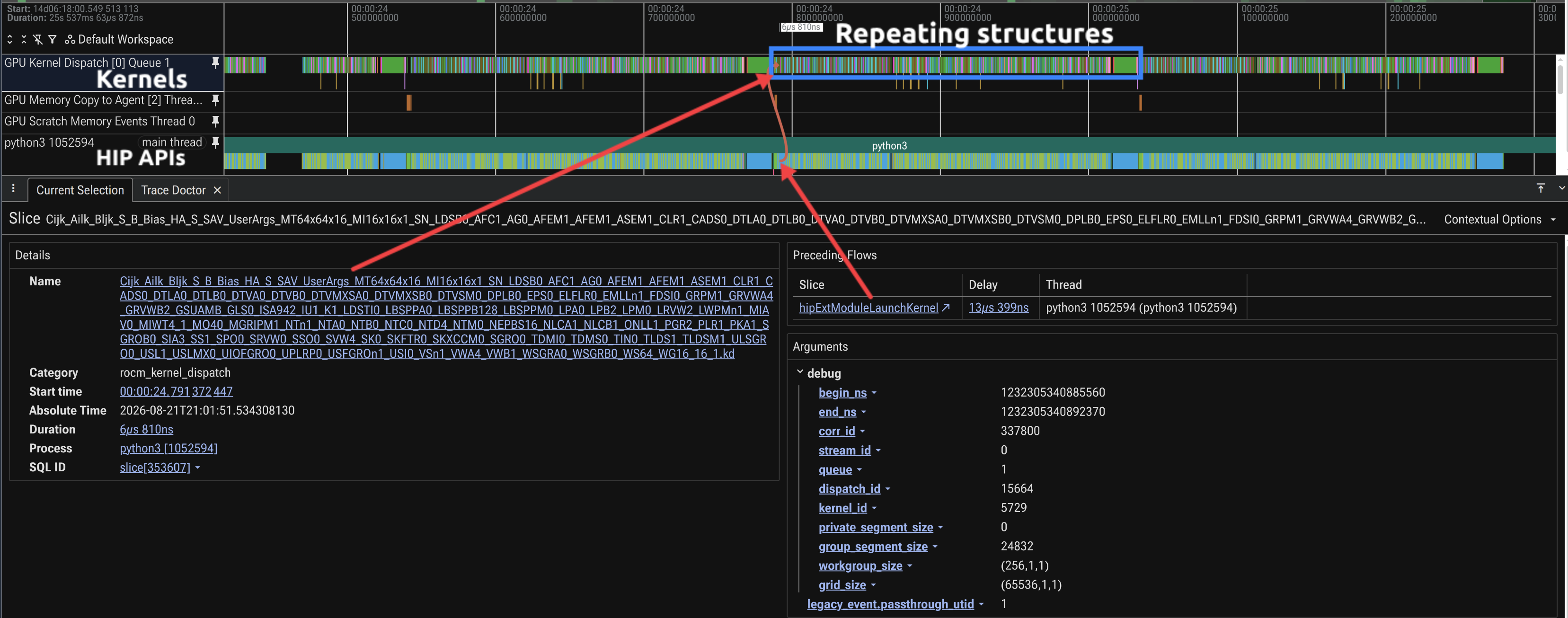
Figure 1b: Zoomed single step of the same trace shows many short kernels with launch gaps between them without phase labels.

Annotate Workload Phases (ROCTx)

To make the trace readable, mark the phases of a training step with ROCTx ranges. From Python, ROCm records torch.cuda.nvtx ranges as ROCTx regions. Wrap the forward and backward passes (and any stage of interest, such as the attention or triangle blocks) with start and stop markers:

import torch

for step in range(num_steps):
    fwd = torch.cuda.nvtx.range_start("forward_pass")
    loss = model(batch)
    torch.cuda.nvtx.range_end(fwd)

    bwd = torch.cuda.nvtx.range_start("backward_pass")
    loss.backward()
    torch.cuda.nvtx.range_end(bwd)
    optimizer.step(); optimizer.zero_grad()

Re-run the same rocprof-sys-run capture on the annotated tiny_openfold_v1_roctx.py:

rocprof-sys-run --rocm=kernel,marker -T -o rsys_v1_annot -- \
  python3 tiny_openfold_v1_roctx.py --batch-size 4 --seq-len 64 --num-seqs 16 --num-blocks 4 --num-steps 10 --device 0

In the resulting Perfetto trace (rsys_v1_annot/<timestamp>/perfetto-trace-*.proto), the named ranges appear in the timeline with the GPU kernels of each phase underneath, which turns the dense baseline trace into a per-phase breakdown.

The key takeaway from the annotated ranges, visible as the two labeled bands in Figure 2 below, is the split between the forward and backward passes. For TinyOpenFold the backward pass is roughly 55–60% of the step, so any optimization that touches both passes (like the fusion in version 2) compounds. The trace also localizes where that cost is incurred, since the triangle and transition general matrix multiplications (GEMMs) dominate, which bounds what later optimizations can achieve (see version 3).

Figure 2: ROCTx-annotated version 1 trace (rocprof-sys-run) with forward_pass and backward_pass bands.

Narrow the Capture (--selected-regions)

With phases labeled, the trace can be restricted to the region of interest instead of recording every step. rocprof-sys-run keeps only the ROCTx ranges named through the --selected-regions flag, turning the dense whole-run timeline into a focused view of, say, the forward and backward passes:

rocprof-sys-run --rocm=kernel,marker --selected-regions=forward_pass,backward_pass -T -o rsys_v1_sel -- \
  python3 tiny_openfold_v1_roctx.py --batch-size 4 --seq-len 64 --num-seqs 16 --num-blocks 4 --num-steps 10 --device 0

The resulting trace contains only the forward_pass and backward_pass regions, and the region names must match the start and stop ROCTx markers added above. The same regions can instead be set through the ROCPROFSYS_SELECTED_REGIONS=forward_pass,backward_pass environment variable. Figure 3 below shows the result, the same capture as Figure 2 with the data-loading and optimizer steps dropped, so the two phases of interest fill the timeline.

Figure 3: The same trace narrowed to forward_pass and backward_pass via --selected-regions.

Device Summary (rocprofv3)

The same region narrowing is available in rocprofv3 for the kernel summary, so the hotspot percentages reflect the phases of interest rather than the whole run. We start with the full-run summary and then narrow it.

ROCR_VISIBLE_DEVICES=0 rocprofv3 --kernel-trace --stats -S -T -d out_v1 -o tinyfold -- \
  python3 tiny_openfold_v1.py --batch-size 4 --seq-len 64 --num-seqs 16 --num-blocks 4 --num-steps 10

On ROCm 7.13 the --stats data lands in the rocpd database (out_v1/tinyfold_results.db) rather than a standalone CSV. Export the aggregated table from that database with rocpd2summary:

rocpd2summary -i out_v1/tinyfold_results.db -f csv -d out_v1/csv -o tinyfold_summary

This writes out_v1/csv/tinyfold_summary_kernels_summary.csv with one row per kernel (name, calls, total/avg duration, and percent of GPU time), the same numbers -S prints. Sorting by GPU time gives the baseline hot spots for the small problem:

Kernel	Calls	Total (ms)	% of GPU time
vectorized_elementwise_kernel	19,468	84.4	26.5%
elementwise_kernel_manual_unroll	4,575	53.8	16.9%
rocBLAS GEMM (Cijk_… MT32x16x128)	1,800	31.1	9.7%
rocBLAS GEMM (Cijk_… MT128x64x32)	1,275	17.3	5.4%
layer_norm_grad_input_kernel	780	14.6	4.6%

The summary exhibits a characteristic shape. The top slots are occupied by the elementwise and tail kernels, which represent the launch-bound fragmentation that results from nothing being fused (note the 19,468 and 4,575 call counts over the 15 executed steps, 10 measured plus 5 warmup). Beneath them sit the rocBLAS Cijk_… GEMMs, the compute-bound triangle and transition matmuls. It is precisely that fragmentation which version 2 targets.

rocprofv3 --selected-regions narrows the summary to the forward and backward passes, but it keys on roctxProfilerResume() and roctxProfilerPause() calls rather than region names. Collection therefore stays off until the first resume call is reached. The annotated variant tiny_openfold_v1_roctx_selected.py wraps the same two spans with those calls (the roctx module ships with the SDK that should be prepended to PYTHONPATH):

import roctx
tid = roctx.getThreadId()

for step in range(num_steps):
    fwd = torch.cuda.nvtx.range_start("forward_pass")
    roctx.profilerResume(tid)      # collection ON
    loss = model(batch)
    roctx.profilerPause(tid)       # collection OFF
    torch.cuda.nvtx.range_end(fwd)

    bwd = torch.cuda.nvtx.range_start("backward_pass")
    roctx.profilerResume(tid)
    loss.backward()
    roctx.profilerPause(tid)
    torch.cuda.nvtx.range_end(bwd)
    optimizer.step(); optimizer.zero_grad()

Because only those two phases are collected, a few steps suffice:

rocprofv3 --selected-regions --kernel-trace --stats -S -T -d out_v1_sel -o selreg -- \
  python3 tiny_openfold_v1_roctx_selected.py --batch-size 4 --seq-len 64 --num-seqs 16 --num-blocks 4 --num-steps 3 --device 0

Narrowing drops the data-loading, optimizer, and warm-up kernels (about 48% of dispatches), so the --stats percentages now describe the forward/backward mix alone, not the whole GPU run. However, the whole-run table above remains the reference for the overall hotspot distribution. Sorting the narrowed summary by GPU time within those phases (Cijk_* GEMM tiles grouped into one bucket) reorders the picture:

Kernel	Calls	Total (µs)	% of GPU time (fwd+bwd)
rocBLAS GEMM (Cijk_*, all tiles)	1,683	24,275	40.1%
vectorized_elementwise_kernel	2,895	15,262	25.2%
elementwise_kernel_manual_unroll	915	10,876	18.0%
layer_norm_grad_input_kernel	156	2,961	4.9%
vectorized_layer_norm_kernel	156	2,440	4.0%

With the loader and optimizer kernels excluded, the triangle/transition GEMMs rise to the top at 40.1% of forward and backward time instead of the elementwise tail. This confirms that the GEMMs are the dominant compute inside the phases that matter, while the elementwise kernels remain the launch-bound overhead that fusion targets.

Identify the Bottleneck

Two distinct signals in the profile point toward the next optimization to apply. The gaps between the many short kernels expose host-side launch overhead, and the HBM traffic from hardware counters quantifies memory movement, both of which fusion (version 2) reduces. We therefore begin by examining the hardware counters for the hottest kernel.

Analyze Hardware Usage (rocprof-compute)

Sorting kernels by time shows where the time goes, whereas the hardware counters show how a kernel uses the GPU. The next step is to collect the full counter set for a top kernel identified in the rocprofv3 summary. When done naively, this re-runs the application once per counter group (dozens of passes); --iteration-multiplexing avoids that by cycling the counters over the kernel’s many calls within a single run. We collect the full counters for the top elementwise kernel and then analyze specific metric blocks.

rocprof-compute profile -n tinyfold_v1_vecelem_mux --device 0 \
  --iteration-multiplexing kernel_launch_params -k vectorized_elementwise_kernel -- \
  python3 tiny_openfold_v1.py --batch-size 4 --seq-len 64 --num-seqs 16 --num-blocks 4 --num-steps 3 --device 0
rocprof-compute analyze -p workloads/tinyfold_v1_vecelem_mux/MI300X_A1 -b 2.1.14 2.1.16 7.1 11.2 17.3 --view table

The -n argument names the workload and -k restricts collection to the matching kernel; results land under workloads/tinyfold_v1_vecelem_mux/<device-arch>/ (for example MI300X_A1). The -b blocks select the metrics of interest: wavefront occupancy (2.1.16) and VALU active threads (2.1.14); wavefront launch stats such as total wavefronts, VGPR, SGPR, and LDS per workgroup (7.1); compute-throughput utilization including VALU utilization and IPC (11.2); and L2 cache bandwidth and hit rate (17.3). We revisit these numbers for version 2 to see what fusion does to this kernel. The complete set of block IDs can be printed with rocprof-compute profile --list-available-metrics, as described in the block filtering documentation.

Step 2 — Optimize with PyTorch Kernel Fusion (Version 2)

The baseline established two facts, namely that many small kernels fragment the step and that the backward pass dominates. Version 2 addresses the fragmentation without leaving PyTorch. All of the commands in this section are run from inside the version2_pytorch_fused/ directory.

What Version 2 Changed and Why

Version 2 keeps the Evoformer math identical but restructures three hot spots so that the framework dispatches fewer, larger kernels:

• MSA QKV fusion — the separate query, key, and value projections become a single combined projection (3 kernels → 1). One larger GEMM does the work of three small ones, cutting launch overhead and giving the GPU a more efficient matrix shape.

• Flash-Attention-style attention — this path avoids materializing the full attention matrix in HBM, which removes a round trip through memory for the largest intermediate tensors.

• Triangle gate/projection fusion — this merge combines the gate and projection of each triangle stage (4 kernels → 2), again replacing several small launches with fewer, larger ones.

This restructuring also lowers the activation footprint of the step. Because the fused attention never materializes the full N×N attention matrix in HBM, version 2’s peak memory drops about 14% below version 1, on top of the throughput gain shown later in this section.

Verify with rocprofv3 and rocprof-sys

We first run the same baseline timing as before.

ROCR_VISIBLE_DEVICES=0 python3 tiny_openfold_v2.py --batch-size 4 --seq-len 64 --num-seqs 16 --num-blocks 4 --num-steps 30

For the small problem, version 2 reports about 229 samples/sec (17.4 ms per batch), a +131% improvement over version 1 (roughly 2.3×), and at lower peak memory. This is the peak of these versions, and it comes entirely from dispatching fewer, larger kernels. Because version 2 is already hand-fused, adding --enable-torch-compile moves it only to about 239 samples/sec and the compiler has little launch overhead left to remove:

Small problem	eager	+ torch.compile
Version 1 baseline	99	174
Version 2 fused	229 (+131%)	239

Now re-run rocprofv3 with the same discipline as version 1 and compare:

ROCR_VISIBLE_DEVICES=0 rocprofv3 --kernel-trace --stats -S -T -d out_v2 -o tinyfold -- \
  python3 tiny_openfold_v2.py --batch-size 4 --seq-len 64 --num-seqs 16 --num-blocks 4 --num-steps 10

To see the QKV fusion rather than infer it from counts, capture a rocprof-sys-run trace of each version with the msa_qkv ROCTx region labeled, then zoom to that band in Perfetto. Both regions are already annotated in the *_roctx.py variants:

ROCR_VISIBLE_DEVICES=0 rocprof-sys-run --rocm=kernel,marker -T -o rsys_v1_qkv -- \
  python3 ../version1_pytorch_baseline/tiny_openfold_v1_roctx.py --batch-size 4 --seq-len 64 --num-seqs 16 --num-blocks 4 --num-steps 5 --device 0

ROCR_VISIBLE_DEVICES=0 rocprof-sys-run --rocm=kernel,marker -T -o rsys_v2_qkv -- \
  python3 tiny_openfold_v2_roctx.py --batch-size 4 --seq-len 64 --num-seqs 16 --num-blocks 4 --num-steps 5 --enable-all-fusion

Open the resulting rsys_v{1,2}_qkv/<timestamp>/perfetto-trace-*.proto files and navigate to the msa_qkv region in each. The contrast is the fusion itself, as Figure 4a below shows the three separate query, key, and value GEMM launches in version 1, and Figure 4b shows the same region in version 2 after they collapse into a single wider GEMM.

Figure 4a: Version 1 msa_qkv region—three separate Q/K/V GEMM launches.

Figure 4b: Version 2 msa_qkv region—the three projections fused into one GEMM.

The trace confirms the kernel count dropped and time moved into a smaller set of larger kernels. On MI300X the total launches per step fall from roughly 3,700 to about 1,700, a ~54% reduction at matched accuracy (see the table below). Most of the reduction comes from the fused attention and triangle projections, which collapse many small launches into a few larger ones; the untouched GEMMs and elementwise tail account for the rest.

The per-step totals below are counted from the rocpd database (rocpd summary over each version’s _results.db, divided by the step count). Version 2’s fusion nearly halves the launch count, corroborating its throughput win:

Version	Kernel launches / step	vs V1
Version 1	3,702	—
Version 2	1,697	−54%

Sorting the version 2 summary by GPU time shows the shift directly:

Kernel	Calls	Total (ms)	% of GPU time
vectorized_elementwise_kernel	5,820	12.9	7.1%
bwd_kernel_fuse (fused Flash-Attention backward)	240	12.8	7.0%
rocBLAS GEMM (Cijk_… MT32x16x128)	600	10.8	5.9%
rocBLAS GEMM (Cijk_… MT128x64x32)	675	9.2	5.1%
rocBLAS GEMM (Cijk_… MT64x32x64)	240	8.9	4.9%

Compared with version 1, the elementwise tail has collapsed. The vectorized_elementwise_kernel entry drops from 19,468 calls/84.4 ms (26.5%) to 5,820 calls/12.9 ms (7.1%), so time is now spread more evenly and the profile is GEMM-dominated (three Cijk_… matmuls in the top five). The bwd_kernel_fuse entry represents the fused Flash-Attention backward kernel, which has relatively few launches (240) but a high computational cost per call.

What fusion does not touch are the triangle and transition GEMMs, which are already efficient rocBLAS calls. After version 2 those GEMMs are what remain, and that sets up the more nuanced lesson of version 3.

Confirm Kernel Fusion Saves Memory

Kernel fusion also lowers the activation footprint of each step. The metric that shows it is peak device allocation (torch.cuda.max_memory_allocated), which captures the intra-step activation high-water mark that fusion changes. The --enable-memory-profiling flag reports this value in the training summary. We run version 1 and version 2 at matched configuration.

ROCR_VISIBLE_DEVICES=0 python3 tiny_openfold_v1.py --batch-size 4 --seq-len 64 --num-seqs 16 --num-blocks 4 --num-steps 30 --device 0 --enable-memory-profiling
ROCR_VISIBLE_DEVICES=0 python3 tiny_openfold_v2.py --batch-size 4 --seq-len 64 --num-seqs 16 --num-blocks 4 --num-steps 30 --enable-all-fusion --enable-memory-profiling

Run	Speed (samples/sec)	Peak memory (max_memory_allocated)	vs V1
Version 1 baseline	97	2,266.9 MB	—
Version 2 (all fusion)	236	1,941.2 MB	−14.4%
Version 2 (--disable-all-fusion, control)	102	2,266.9 MB	0.0%

These speeds are a separate run from the timing numbers above.

Kernel fusion cuts peak memory 14.4% (−326 MB), because the Flash-Attention-style attention never materializes the full N×N attention matrix and so lowers the activation high-water mark. The --disable-all-fusion control lands byte-for-byte on version 1’s peak, which proves the saving comes from the fusion itself and not from version 2 being a different script.

Confirm the Effect at the Counter Level

The kernel-count table showed fusion cut launches; the hardware counters show what it did to the one elementwise kernel that survives in both versions. Re-run the same full-counter capture from Step 1 on version 2 and compare the two:

rocprof-compute profile -n tinyfold_v2_vecelem_mux --device 0 \
  --iteration-multiplexing kernel_launch_params -k vectorized_elementwise_kernel -- \
  python3 tiny_openfold_v2.py --batch-size 4 --seq-len 64 --num-seqs 16 --num-blocks 4 --num-steps 3 --enable-all-fusion
rocprof-compute analyze -p workloads/tinyfold_v2_vecelem_mux/MI300X_A1 -b 2.1.14 2.1.16 7.1 11.2 17.3 --view table

Metric (vectorized_elementwise_kernel)	Version 1	Version 2	Change
Total wavefronts (max)	16,384	8,192	½ the waves
L2 cache bandwidth achieved (avg, Gb/s)	1,496	3,152	~2.1× higher
L2 cache hit rate (%)	44.4	51.5	+7 points
VALU utilization (%)	0.43	0.18	lower per call
Wavefront occupancy (avg)	203.6	108.9	lower
IPC issued	1.02	1.00	~same

Kernel fusion halves the wavefronts launched for the elementwise tail and drives about 2.1× higher L2 bandwidth utilization with a +7-point cache hit rate on the kernel that remains, the same work done in fewer, better-fed dispatches that hit cache more often. Taken together, these counters constitute the evidence behind version 2’s throughput gain. (Iteration-multiplexing metrics come from partially available counter data and are best read as relative comparisons, not absolute values.)

It should be noted that this is not a strict one-to-one kernel comparison. Kernel fusion absorbs the FP32 elementwise work (bias-add, gating, activations) into the fused attention/GEMM kernels, so version 2’s standalone elementwise tail is a different, smaller set of kernels than version 1’s, and the counters compare the tail as a whole, not an identical kernel.

Step 3 — Optimize with Triton Kernels (Version 3)

Version 2 removed the launch overhead and reached the throughput peak. Version 3 adds custom Triton kernels, and in doing so demonstrates a central principle, namely that a hand-written kernel helps only when it targets where the time is actually spent. All of the commands in this section are run from inside the version3_triton/ directory.

What Version 3 Changed and Why

• Fused LayerNorm — a single Triton kernel computes mean, variance, normalization, and the affine scale in one pass over the data, instead of several PyTorch ops each reading and writing HBM.

• Fused attention (SDPA) + QKV fusion — attention uses PyTorch’s fused scaled-dot-product attention (a real flash-attention kernel) with the query/key/value projections combined, each wrapped in a torch.autograd.Function so gradients flow correctly.

Both of these are memory-bound operations, and that fact is the crux of the matter. The model spends most of its time in the triangle and transition GEMMs, identical rocBLAS calls in all three versions that version 3 does not touch. Customizing the memory-bound LayerNorm and attention optimizes a small slice of the total runtime.

Warm Up Before Measuring

Triton compiles and autotunes its kernels on first use. A cold first step is far slower than steady state and would unfairly penalize version 3. We therefore run the project’s correctness check (python3 test_correctness.py) and then take enough warmup steps to populate the Triton cache before recording any timing or counters.

ROCR_VISIBLE_DEVICES=0 python3 tiny_openfold_v3.py --batch-size 4 --seq-len 64 --num-seqs 16 --num-blocks 4 --num-steps 30

The measured result constitutes the central lesson of this section. For the small problem, eager version 3 reports about 91 samples/sec (44.1 ms per batch), roughly 0.9× version 1, that is, slightly slower than the readable baseline, and well below version 2’s 229 samples/sec. Two effects offset one another here. The QKV fusion and fused SDPA reduce launch overhead, but wrapping each custom Triton kernel in a torch.autograd.Function adds approximately 0.1 ms per call, and across the ~36 LayerNorm calls per step this Python overhead roughly cancels the savings. Optimizing a memory-bound slice of a GEMM-bound model cannot, on its own, move end-to-end time appreciably.

The custom kernels do pay off once the compiler removes that per-call overhead. When --enable-torch-compile is added, inductor fuses the graph around the custom kernels, though it still calls the Triton LayerNorm rather than replacing it.

ROCR_VISIBLE_DEVICES=0 python3 tiny_openfold_v3.py --batch-size 4 --seq-len 64 --num-seqs 16 --num-blocks 4 --num-steps 30 \
  --enable-torch-compile

Compiled version 3 reaches about 196 samples/sec (~2.2× over eager V3), which finally edges past compiled version 1 (~174 samples/sec) at the small problem, but still sits below version 2, and the edge does not hold at the large problem (see the final comparison table). The lesson is to always measure against the compiled baseline, not just eager, and not to assume a hand-written kernel wins until measurement says so.

Verify with rocprofv3 and rocprof-compute

ROCR_VISIBLE_DEVICES=0 rocprofv3 --kernel-trace --stats -S -T -d out_v3 -o tinyfold -- \
  python3 tiny_openfold_v3.py --batch-size 4 --seq-len 64 --num-seqs 16 --num-blocks 4 --num-steps 10

Expect new kernel-name patterns, since the Triton and SDPA kernels will not match the aten::-derived names from versions 1 and 2. The summary can be filtered with -T and substring matching. Sorting the version 3 summary by GPU time gives:

Kernel	Calls	Total (ms)	% of GPU time
vectorized_elementwise_kernel	14,885	72.5	24.2%
elementwise_kernel_manual_unroll	6,435	67.6	22.5%
rocBLAS GEMM (Cijk_… MT32x16x128)	1,080	19.8	6.6%
reduce_kernel	1,095	16.1	5.4%
rocBLAS GEMM (Cijk_… MT128x64x32)	915	12.4	4.1%
…
layernorm_dx_kernel (Triton bwd, rank 10)	780	9.5	3.2%
layernorm_kernel (Triton fwd, rank 11)	780	9.0	3.0%

The two custom Triton LayerNorm kernels are version-3-specific contributions that rank below the top five kernels. Together, they account for only approximately 6% of GPU time. This is the point at which the profiler explains the throughput result. Unlike version 2, whose fusion collapsed the elementwise tail (vectorized_elementwise_kernel fell from 19,468 calls/84.4 ms to 5,820 calls/12.9 ms), eager version 3 still looks like version 1, in that the same elementwise kernels top the list, because version 3 only touches the memory-bound LayerNorm and attention, not the elementwise and GEMM bulk. The custom Triton kernels appear lower at roughly 9 ms each, and the triangle and transition GEMMs still dominate, unchanged from versions 1 and 2. That is why customizing those kernels barely moves the total, and it shows in the launch count. Eager version 3 leaves the elementwise and GEMM bulk untouched, so its per-step total stays near version 1:

Version	Kernel launches / step	vs V1
Version 1	3,702	—
Version 2	1,697	−54%
Version 3	3,285	−11%

To judge the custom kernel on its own terms, compare it head-to-head with the native kernel it replaced using the same full-counter workflow. The LayerNorm input-gradient exists in both versions (the Triton layernorm_dx_kernel in version 3 and the native layer_norm_grad_input_kernel in version 1), so profiling each with rocprof-compute at identical grid and wave count gives a fair per-dispatch comparison:

# Version 3: the Triton input-gradient kernel
rocprof-compute profile -n tinyfold_v3_roof_dx --device 0 --roof-only -k layernorm_dx_kernel -- \
  python3 tiny_openfold_v3.py --batch-size 4 --seq-len 64 --num-seqs 16 --num-blocks 4 --num-steps 10

# Version 1: the native input-gradient kernel (run from version1_pytorch_baseline/)
rocprof-compute profile -n tinyfold_v1_lngrad --device 0 --roof-only -k layer_norm_grad_input_kernel -- \
  python3 tiny_openfold_v1.py --batch-size 4 --seq-len 64 --num-seqs 16 --num-blocks 4 --num-steps 10 --device 0

Metric (mean / dispatch)	V3 Triton layernorm_dx_kernel	V1 native layer_norm_grad_input_kernel	ratio (V3/V1)
Vector general-purpose registers (VGPR) / wave	12	24	0.50×
Local data share (LDS) / workgroup (bytes)	8	16	0.50×
Active GPU cycles (GRBM)	264,138	404,504	0.65×
VALU F32 instructions	1,855,173	1,354,675	1.37×
LDS-active cycles	725,937	3,498,614	0.21×
Total cache accesses	700,731	2,681,938	0.26×
HBM read + write requests	108,647 / 95,783	109,082 / 95,783	~1.00×

The Triton kernel is genuinely more efficient per dispatch, with about 35% fewer active GPU cycles and roughly half the VGPR and LDS per wave. Its standout win is ~4–5× fewer LDS-active cycles and cache accesses (0.21×/0.26×), because the single-pass Triton LayerNorm keeps intermediates in registers instead of round-tripping through LDS and cache like the native multi-op path. It executes ~1.37× more VALU F32 instructions (the fused recompute), but that is cheap next to the cache and LDS savings. HBM traffic is essentially identical (~1.00×), as expected for a memory-bound op that must move the same bytes either way.

[!Note] Two caveats on this table. First, these are two different kernels performing the same operation, not one kernel measured twice, since version 1 has no Triton kernel and version 3 replaced the native one, so a cross-implementation comparison is the only option. Second, it covers only the input-gradient (∂/∂x); PyTorch splits the full LayerNorm backward across additional kernels (the weight and bias gradients), which are not included here.

The custom kernel wins every counter that matters for a memory-bound op, yet it is only ~3% of GPU time, so those wins cannot move end-to-end throughput. The hardware counters explain why the big lever was fusion (version 2), not custom kernels.

Iterate and Compare Versions Fairly

A profiling comparison is only meaningful if the two runs are otherwise identical. Before comparing any two versions:

• Fix batch size, sequence length, MSA depth (--num-seqs), block count, automatic mixed precision (AMP) mode, and step count across all runs.

• Pin a single device (ROCR_VISIBLE_DEVICES=0 or --device 0) so timing is deterministic.

• For version 3, separate warmup from measurement, and never compare a Triton cold start against a steady version 1 step.

• Give each rocprof-compute run a distinct workload name (tinyfold_v1_mux, tinyfold_v2_mux, tinyfold_v3_mux) so compare mode does not mix stale directories.

With matched configurations, the story is consistent across problem sizes. Version 2 fusion is the peak, eager version 3 sits near or just below version 1, and torch.compile gives roughly 1.4–2.2× on version 1 and version 3 (adding little to the already-fused version 2). All numbers are samples/sec on MI300X / ROCm 7.13[1]:

Problem		Version 1	Version 2	Version 3
Small (64 res, 16 MSA, batch 4)	eager	99	229 (+131%)	91 (−8%)
	+ torch.compile	174	239	196
Large (128 res, 32 MSA, batch 4)	eager	63	106 (+68%)	64 (+2%)
	+ torch.compile	95	106	91

Two profiling lessons follow directly from this table. First, the largest lever was framework-level fusion rather than the hand-written kernels, because fusion reduced launch overhead across the entire step, whereas the custom kernels addressed only a memory-bound slice of a GEMM-bound model. Second, one should always compare against the compiled baseline. Eager version 3 appears to regress, yet compiled version 3 edges past compiled version 1 at the small problem. The operative regime (launch-bound or compute-bound) determines how much any optimization can yield, and only measurement can establish which regime applies.

To produce a side-by-side rocprof-compute report between two versions, collect a full counter set for each (as shown above) and pass both workloads to analyze, as in the advanced article. If a hot kernel was renamed by fusion or Triton, match by dispatch order or a broader -k substring rather than an exact name.

Compare the Runtime Traces Across Versions

The baseline system trace showed a fragmented step; the payoff is seeing that fragmentation shrink after fusion. We re-run the same rocprof-sys-run capture with the --selected-regions narrowing from the baseline section on version 2 (and version 3), keeping the configuration identical, and reuse the annotated *_roctx.py variants so that the forward_pass and backward_pass regions are directly comparable.

ROCR_VISIBLE_DEVICES=0 rocprof-sys-run --rocm=kernel,marker --selected-regions=forward_pass,backward_pass -T -o rsys_v2_sel -- \
  python3 tiny_openfold_v2_roctx.py --batch-size 4 --seq-len 64 --num-seqs 16 --num-blocks 4 --num-steps 10

ROCR_VISIBLE_DEVICES=0 rocprof-sys-run --rocm=kernel,marker --selected-regions=forward_pass,backward_pass -T -o rsys_v3_sel -- \
  python3 tiny_openfold_v3_roctx.py --batch-size 4 --seq-len 64 --num-seqs 16 --num-blocks 4 --num-steps 10

Each resulting Perfetto trace (rsys_v{2,3}_sel/<timestamp>/perfetto-trace-*.proto) can be opened at https://ui.perfetto.dev/ alongside the version 1 capture from the baseline section. Figures 5a, 5b, and 5c below show the same forward_pass and backward_pass regions across all three versions at matched configuration, making the structural difference apparent from the timeline shape. Figure 5a is the fragmented version 1 baseline, Figure 5b is the fused version 2, and Figure 5c is eager version 3.

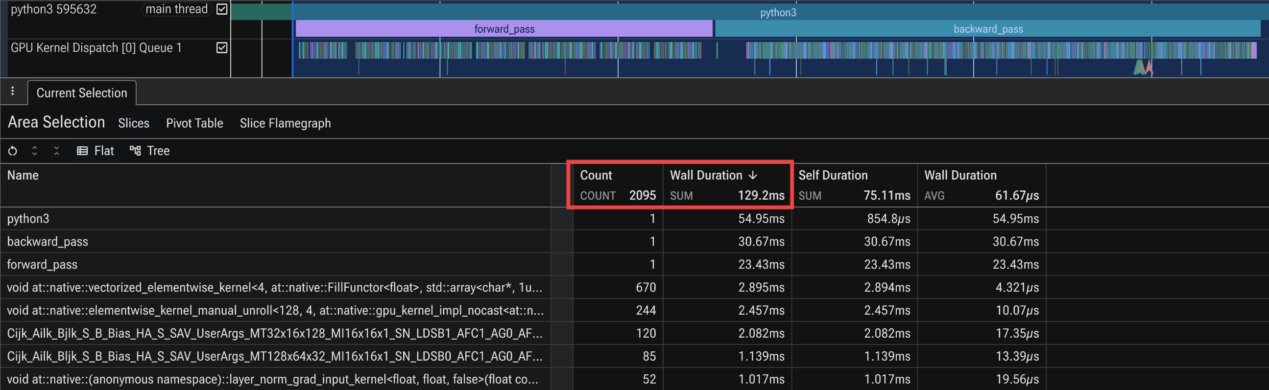
Figure 5a: Version 1 forward/backward passes—many short kernels with launch gaps.

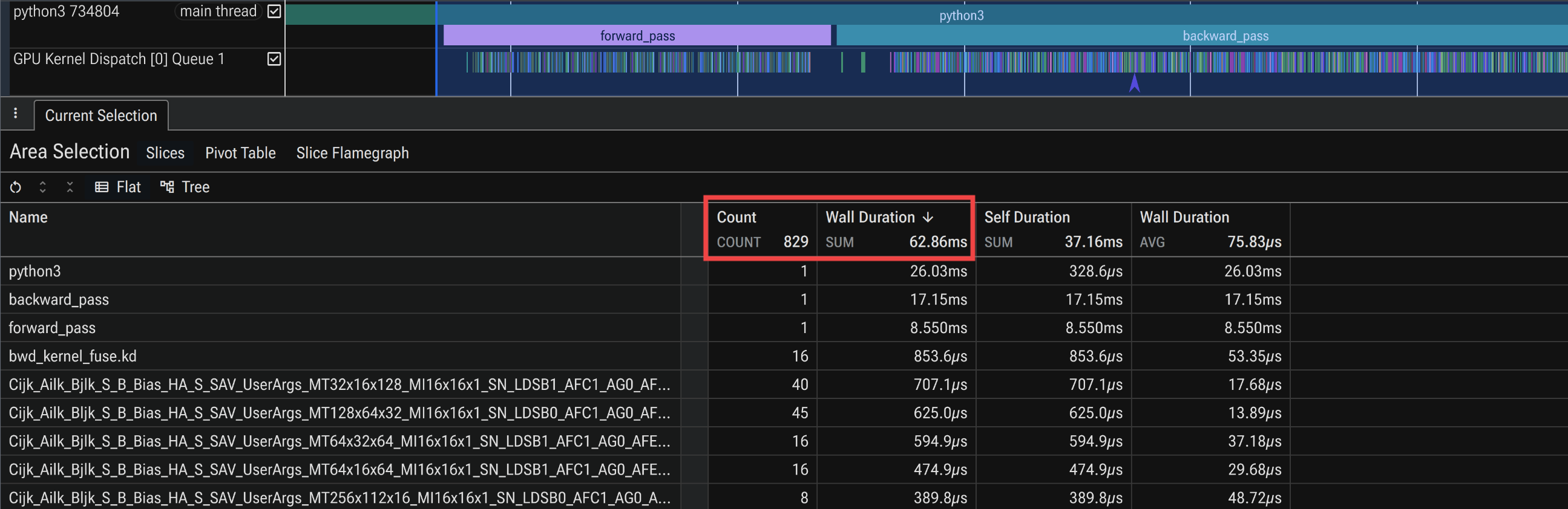
Figure 5b: Version 2—fewer, longer kernels and a visibly shorter region.

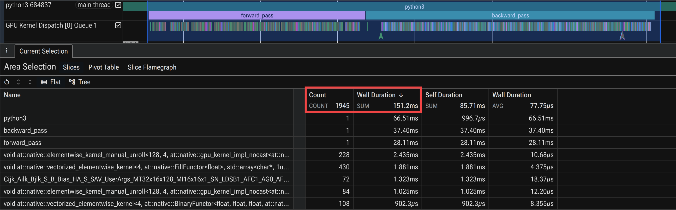
Figure 5c: Eager version 3—fragmentation returns, resembling version 1 more than version 2.

The comparison renders the article’s central result in visual form. Version 2 fusion is the only change that shrinks both the kernel count and the wall-clock width of the region. Version 1 and eager version 3 look alike, dense with short launches and gaps, while version 2 stands out with fewer, longer kernels and a narrower span, matching the throughput numbers and the kernel-count deltas measured earlier.

Because it is a system trace, it also indicates when the GPU is the wrong place to look. A timeline that shows the GPU idle between bursts of kernels points to a host bottleneck (Python overhead, the data pipeline, or synchronization), and correlating the Python/process threads, HIP runtime, and GPU rows in one view separates a host-bound stall from a device-bound stretch. The same trace is the right starting point for extending TinyOpenFold to data-parallel multi-GPU runs, where collectives must be distinguished from compute; the advanced article walks through merging per-rank traces.

Summary

This post applied the ROCm profiling toolchain to a PyTorch training workload. ROCm Systems Profiler (rocprof-sys) captured a whole-run system trace with its workload-trace preset, and rocprofv3 produced a kernel summary, together exposing the bottleneck, a step broken down into thousands of small kernel launches on top of GEMM-bound triangle compute. Both tools support --selected-regions to narrow collection to the phases of interest (forward and backward); restricting the summary this way removed the loader and optimizer noise and showed the triangle and transition GEMMs as the true hotspot inside those phases. ROCm Compute Profiler (rocprof-compute) then quantified each optimization using hardware counters, its iteration-multiplexing option collecting the full counter set in a single pass and substantially reducing both the profiling time and the on-disk footprint.

The measurements obtained from these tools guided the work directly. PyTorch fusion (version 2) roughly halved the launches per step for a ~2.3× gain while also cutting peak memory ~14%, confirmed by fewer wavefronts and higher cache bandwidth on the surviving kernels, and proved to be the throughput peak. Custom Triton kernels (version 3) targeted memory-bound operations that were only a small share of a GEMM-dominated step, so eager version 3 matched the baseline and overtook it only under torch.compile at the small problem, an orthogonal optimization that added a ~1.4–2.2× gain to version 1 and version 3 (and little to the already-fused version 2).

The lesson is to profile before optimizing, and measure against the compiled baseline. Optimization effort is worth spending only on the hotspot regions the profiler timeline exposes.

Additional Resources

• Performance Profiling on AMD GPUs Blog Posts:

  • Part 1: Foundations

  • Part 2: Basic Usage

  • Part 3: Advanced Usage

  • Part 4: Fortran OpenMP Offload Edition

  • Part 5: Profiling-Driven Kernel Optimization with an AI Code-Assist Tool

  • Part 6: Advanced Thread Trace (ATT) - The Microscope for Your Application

• TinyOpenFold example and tutorial:

  • TinyOpenFold in HPCTrainingExamples

  • Performance Optimization Tutorial

  • ARCHITECTURE.md

• OpenFold / AlphaFold 2:

  • OpenFold

  • Jumper et al., Highly accurate protein structure prediction with AlphaFold, Nature 2021

• Perfetto UI:

  • Online documentation for using Perfetto UI

• ROCm Optiq:

  • What is ROCm Optiq?

  • Open source at Optiq github repo

• rocprofiler-sdk:

  • Open source at rocprofiler-sdk github repo

  • rocprofiler-sdk documentation

  • rocprofv3 documentation

• rocprof-compute:

  • Open source at rocprofiler-compute github repo

  • ROCm Compute Profiler documentation

• rocprof-sys:

  • Open source at rocprofiler-systems github repo

  • ROCm Systems Profiler documentation

• PyTorch for ROCm:

  • PyTorch on ROCm documentation

  • Triton documentation

If you have any questions or comments, please reach out to us on GitHub Discussions.

Disclaimers

The information presented in this document is for informational purposes only and may contain technical inaccuracies, omissions, and typographical errors. The information contained herein is subject to change and may be rendered inaccurate for many reasons, including but not limited to product and roadmap changes, component and motherboard version changes, new model and/or product releases, product differences between differing manufacturers, software changes, BIOS flashes, firmware upgrades, or the like. Any computer system has risks of security vulnerabilities that cannot be completely prevented or mitigated. AMD assumes no obligation to update or otherwise correct or revise this information. However, AMD reserves the right to revise this information and to make changes from time to time to the content hereof without obligation of AMD to notify any person of such revisions or changes. THIS INFORMATION IS PROVIDED “AS IS.” AMD MAKES NO REPRESENTATIONS OR WARRANTIES WITH RESPECT TO THE CONTENTS HEREOF AND ASSUMES NO RESPONSIBILITY FOR ANY INACCURACIES, ERRORS, OR OMISSIONS THAT MAY APPEAR IN THIS INFORMATION. AMD SPECIFICALLY DISCLAIMS ANY IMPLIED WARRANTIES OF NON-INFRINGEMENT, MERCHANTABILITY, OR FITNESS FOR ANY PARTICULAR PURPOSE. IN NO EVENT WILL AMD BE LIABLE TO ANY PERSON FOR ANY RELIANCE, DIRECT, INDIRECT, SPECIAL, OR OTHER CONSEQUENTIAL DAMAGES ARISING FROM THE USE OF ANY INFORMATION CONTAINED HEREIN, EVEN IF AMD IS EXPRESSLY ADVISED OF THE POSSIBILITY OF SUCH DAMAGES.

Third-party content is licensed to you directly by the third party that owns the content and is not licensed to you by AMD. ALL LINKED THIRD-PARTY CONTENT IS PROVIDED “AS IS” WITHOUT A WARRANTY OF ANY KIND. USE OF SUCH THIRD-PARTY CONTENT IS DONE AT YOUR SOLE DISCRETION AND UNDER NO CIRCUMSTANCES WILL AMD BE LIABLE TO YOU FOR ANY THIRD-PARTY CONTENT. YOU ASSUME ALL RISK AND ARE SOLELY RESPONSIBLE FOR ANY DAMAGES THAT MAY ARISE FROM YOUR USE OF SUCH THIRD-PARTY CONTENT.

AMD, the AMD Arrow logo, AMD Instinct, ROCm, and combinations thereof are trademarks of Advanced Micro Devices, Inc. Other product names used in this publication are for identification purposes only and may be trademarks of their respective companies.

PyTorch, the PyTorch logo and any related marks are trademarks of The Linux Foundation.

Python is a trademark of the Python Software Foundation.

© 2026 Advanced Micro Devices, Inc. All rights reserved.

---

[1] (1,2)

Throughput numbers (samples/sec and per-batch times) quoted in this post were measured on a single AMD Instinct MI300X (gfx942) with ROCm 7.13 (TheRock nightly: PyTorch 2.11 / Triton 3.6). They are consistent with the upstream TinyOpenFold Performance Optimization Tutorial; the batch-size-4 configuration used here differs from the tutorial’s published runs, so absolute numbers are not expected to match exactly. They illustrate the relative impact of each optimization stage; absolute performance will vary with the GPU model, ROCm and PyTorch versions, problem configuration, and system setup. Reproduce on your own hardware using the commands shown and compare runs only at matched configurations.