Performance Profiling on AMD GPUs - Part 4: Fortran OpenMP Offload Edition

June 01, 2026 by Thomas Gibson, Asitav Mishra, Luka Stanisic, Gina Sitaraman.

12 min read. | 2903 total words.

Software tools & optimizations

HPC, Performance, Optimization, Profiling, Compiler, OpenMP

HPC, Developers

This blog, like the previous articles in the profiling guide series (Part 1, Part 2, and Part 3), is designed to help you systematically analyze and improve the performance of your Fortran OpenMP offload applications running on AMD GPUs. This guide builds upon the foundational skills from the previous articles and introduces profiling techniques specifically tailored for Fortran applications that use OpenMP target offloading.

1. What You Already Know:

   • Your Fortran application leverages OpenMP target offloading to execute computation on AMD GPUs.

   • You understand the basic purpose of OpenMP target regions in your code.

   • You have observed performance bottlenecks or want to optimize your application’s GPU utilization (optional).

2. What This Guide Will Teach You:

   • Fortran OpenMP Profiling Basics: Learn how to profile Fortran applications with OpenMP offload and measure where your application spends time.

   • Multi-Device Profiling: Explore profiling techniques for MPI-based multi-process Fortran applications running on multiple GPUs in a single node.

   • Advanced Analysis: Use ROCm profiling tools to identify bottlenecks in GPU kernels, host-side execution, and data movement patterns.

   • Optimization Strategies: Apply targeted optimizations based on profiling insights to improve performance.

By the end of this blog, you will be able to profile your Fortran OpenMP offload application to identify opportunities for optimization on the GPU, CPU, and in data movement, with a focus on achieving optimal performance on AMD hardware.

This blog uses profilers from ROCm 7.2. Experiments were run on an MI300A APU, which supports the unified memory model, but the methodology described in this blog is general and also applicable to discrete GPUs.

Profiling Basics

We follow the same systematic profiling workflow introduced in the previous articles in the profiling guide series: establish baseline performance, identify bottlenecks (host vs. device vs. data movement), analyze hardware resource usage and kernel performance metrics, perform targeted optimizations, and iterate. For Fortran OpenMP offload applications, this workflow helps identify opportunities to optimize OpenMP target regions, reduce data transfers between host and device, and improve GPU utilization.

The ROCm profiling tools have been successfully demonstrated on simpler Fortran OpenMP offload examples in the HPCTrainingExamples repository. For instance, the rocprofv3 OpenMP examples show how to collect timeline traces, the rocprofiler-systems Jacobi example demonstrates system-level profiling, and the Fortran Jacobi example with ROCTx markers illustrates code instrumentation techniques. Additionally, the rocprof-compute OpenMP Fortran examples demonstrate detailed kernel analysis.

Starting from ROCm 7.0, ROCm profiling tools are being enhanced to write profiled data into a SQLite3-based database in order to decouple post-processing from the profiling stage. Post-processing can now be done using a new tool called rocpd. The advantage of using this workflow is that we profile once and perform several types of analyses on the collected profiled data. This blog demonstrates this “rocprofv3 once + rocpd many times” workflow. Usage instructions and a summary of features of rocpd are documented in the “Using rocpd output format” page. The rocpd training example demonstrates rocpd usage with two Jacobi examples.

For the rest of this blog, we will apply similar methodologies and tooling to a more complex application: GenASiS.

GenASiS Example

As a working example, we will use GenASiS (General Astrophysical Simulation System), a production astrophysics simulation code that combines Message Passing Interface (MPI) for distributed parallelism with OpenMP target offloading for GPU acceleration. Specifically, we use the GenASiS_Basics repository maintained by researchers at Oak Ridge National Laboratory. GenASiS is an excellent example because it represents a real-world HPC workload with complex communication patterns and computational kernels.

GenASiS uses a distributed mesh approach with domain decomposition, making it well-suited for multi-GPU configurations. The application includes various computational kernels for solving conservation equations, performing reconstructions, and computing fluxes; these are typical operations found in many scientific simulation codes. To build GenASiS with OpenMP offload support for AMD GPUs, you will need:

• A Fortran compiler with OpenMP offload support.

• ROCm libraries and runtime.

• An MPI installation compatible with the Fortran toolchain.

While other Fortran compilers support AMD GPU offloading (e.g., HPE Cray Fortran), this blog features the amdflang compiler from AMD. You can obtain amdflang either from the standalone ROCm AFAR pre-production toolchain (see the ROCm AFAR introduction blog) or from the integrated compiler included in ROCm 7.0+ (typically an older version than the pre-production ROCm AFAR releases). For detailed build instructions, see the GenASiS Basics README file. For this blog, GenASiS was compiled using amdflang from ROCm AFAR drop 22.2.0 with -O3 -fopenmp --offload-arch=gfx942, along with OpenMPI 5.0.3.

Single-Device Profiling

Picking the Right Problem Size

To obtain a representative performance profile, choose a problem size that saturates the device’s compute and memory resources. For GenASiS on a node with 4 MI300A devices, running one process per GPU device, a grid of 468 × 468 × 468 cells per device provides a good balance, yielding a memory footprint of approximately 90GB per device. The amount of host and device memory used in an application over time can be traced using rocprofv3, for example, as discussed in Generating Timeline Traces.

Before attaching any profiler, run the application at this size to simultaneously verify correct execution, confirm that OpenMP offloading is active, and record the initial timing statistics from the application’s built-in timers:

mpirun -np 1 GenASiS_Basics/install/bin/RiemannProblem_rocm-afar \
  Verbosity=INFO_2 nCells=468,468,468 Dimensionality=3D FinishCycle=5

If you run under Slurm, use an equivalent srun invocation instead of mpirun.

The output should include OpenMP environment information confirming successful offload:

INFO_1: OpenMP environment
         MaxThreads  =         2
           nDevices  =         4
     OffloadEnabled  =   TRUE
    Selected device  =         0

The OffloadEnabled = TRUE confirms that OpenMP target regions will execute on the GPU. Once correctness is established, we can start analyzing the application’s performance using profiling tools.

Adding ROCTx Markers to Fortran Code

We recommend instrumenting important regions of your code using ROCTx markers before you start profiling. In a Fortran application like GenASiS, ROCTx regions can be added using interfaces in the hipfort library. Here are the steps to follow:

1. Import the hipfort_roctx module at the top of your Fortran source file.

2. Call roctxRangePush at the start of a region you want to annotate (note that this requires a null-terminated string).

3. Call roctxRangePop at the end of the region.

Because hipfort exposes these routines as Fortran interfaces to the C ROCTx API, region names must be explicitly null-terminated on the Fortran side: C expects null-terminated strings, whereas Fortran character strings do not include a terminating null character unless you append it (e.g. with // char(0)).

The following example shows how the main evolution loop in ConservationLawEvolution_Template.f90 is instrumented:

use hipfort_roctx

! ... in your subroutine ...
integer :: iRoctxLevel

do while ( CLE % Time < CLE % FinishTime )
  iRoctxLevel = roctxRangePush ( "EvolveStep" // char(0) )

  ! Nested marker for timestep computation
  iRoctxLevel = roctxRangePush ( "ComputeTimeStep" // char(0) )
  call ComputeTimeStep ( CLE )
  iRoctxLevel = roctxRangePop ( )  !-- ComputeTimeStep
  
  ! Nested marker for conservation law solve
  iRoctxLevel = roctxRangePush ( "CLS_Solve" // char(0) )
  call CLS % Solve ( CLE % TimeStep )
  iRoctxLevel = roctxRangePop ( )  !-- CLS_Solve

  iRoctxLevel = roctxRangePop ( )  !-- EvolveStep
end do

Markers can be nested to show hierarchical structure in the timeline trace as shown in the example above with EvolveStep and ComputeTimeStep regions. The hipfort library is included with standard ROCm installations. When compiling, include the hipfort headers (e.g., -I${ROCM_PATH}/include/hipfort/amdgcn), and when linking, add the rocprofiler-sdk ROCTx library (e.g., -L${ROCM_PATH}/lib -lrocprofiler-sdk-roctx).

Collecting Kernel and ROCTx Region Hotspot Summary

First, we identify which kernels consume the most GPU time and how much time we spend in different ROCTx regions by running rocprofv3 --runtime-trace followed by rocpd summary. Note that options such as --runtime-trace or --sys-trace also collect ROCTx marker regions among others:

mpirun -np 1 \
  rocprofv3 --runtime-trace -d outdir -o genasis_trace -- \
  GenASiS_Basics/install/bin/RiemannProblem_rocm-afar \
  Verbosity=INFO_2 nCells=468,468,468 Dimensionality=3D FinishCycle=5
rocpd summary --region-categories KERNEL MARKER -i outdir/genasis_trace_results.db

The kernel hotspot list reveals a relatively flat profile, where no single kernel dominates execution time. The top 5 kernels account for approximately 50% of GPU time[1]:

Rank	Kernel Name	% GPU Time	Calls	Avg Duration (ms)
1	computeeigenspeedskernel_l166	12.7%	130	2.86
2	computefluxeskernel_l225	10.6%	150	2.07
3	computefluxeskernel_l290	10.6%	150	2.06
4	computeauxiliarykernel_l104	8.4%	130	1.88
5	computeconservedkernel_l19	8.2%	120	2.01

This suggests that we may benefit from optimizations that could be uniformly applied across multiple kernels rather than targeting a single hotspot.

The DURATION column in the markers summary helps you see how much time is spent in each marker region. Note that if there are no nested regions, the PERCENT column can help identify which regions the application spends most time in (not applicable here due to the presence of nested regions).

MARKERS_SUMMARY:
                      Name  Calls  DURATION (nsec)  AVERAGE (nsec)  PERCENT (INC)  MIN (nsec)  MAX (nsec)       STD_DEV
               Computation      1       7034060565    7.034061e+09      13.614240  7034060565  7034060565           NaN
                EvolveStep      5       7034041615    1.406808e+09      13.614203  1393918636  1447001992  2.261686e+07
                 CLS_Solve      5       7030723958    1.406145e+09      13.607782  1393569274  1445174903  2.196855e+07
             ComputeUpdate     10       6714775351    6.714775e+08      12.996272   666099033   688223340  8.433135e+06
<snip>

Generating Timeline Traces

Next, we generate a Perfetto timeline trace to understand execution patterns.

rocpd2pftrace -i outdir/genasis_trace_results.db -d outdir -o genasis_trace 

This command generates a trace file (outdir/genasis_trace_results.pftrace) that can be visualized in the Perfetto UI. Note that the profile we collected previously is used again, this time to generate the Perfetto trace.

When you load the trace in Perfetto, you will first see a high-level view of the application run from the traced marker regions, as shown in Figure 1. The Computation region, which we use to indicate our Figure-Of-Merit (FoM) region, is at the outermost level, with other ROCTx regions nested inside it.

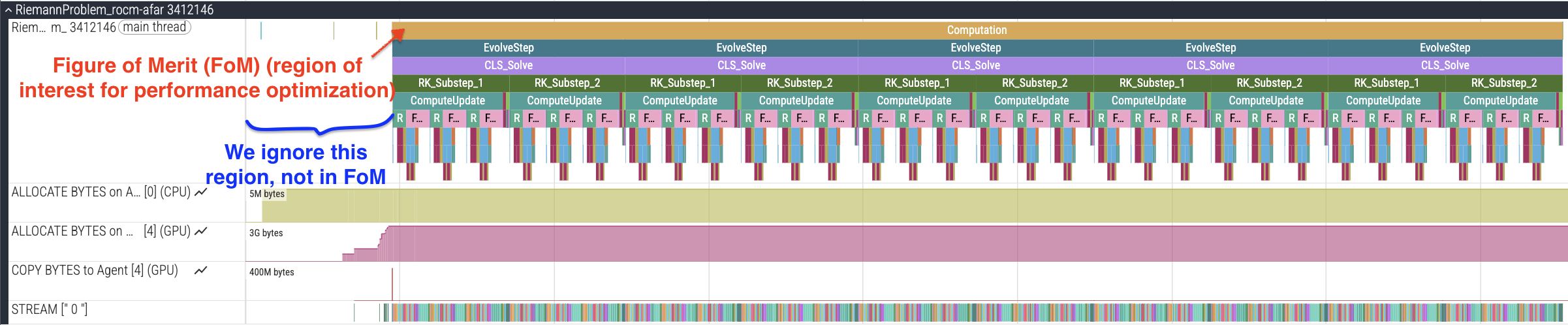
Figure 1: Perfetto trace showing instrumented ROCTx markers and FoM region.

When you zoom in as shown in Figure 2, you will observe several key elements in the timeline trace:

• OMP Activity: OpenMP offload regions appear as GPU kernel dispatches, showing when computation happens on the device. Overlap between compute kernels—or the lack of it—may suggest optimizations.

• Memory allocation: Timeline traces include memory allocation (in bytes) for host and device pools, allowing you to track memory usage in your application.

• Data Movement Patterns: Memory copies between host and device are visible as copy operations. Frequent or large data transfers may become bottlenecks. We can look for unnecessary transfers or for data that could remain on device between iterations.

• Gaps in GPU activity: Timeline traces show periods where the GPU is idle, indicating host-side work or synchronization points. These gaps could lead us to compute regions that could be offloaded to the GPU.

• ROCTx Markers: Custom instrumentation markers (EvolveStep, CLS_Solve, RK_Substep, Communication) provide visibility into major code regions.

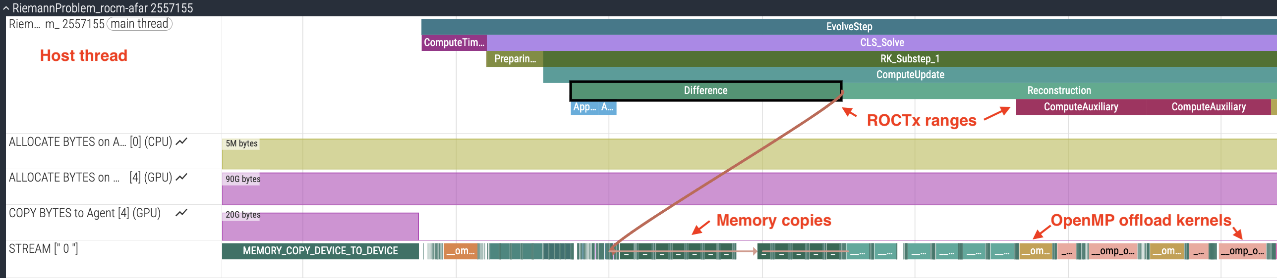
Figure 2: Perfetto trace showing OMP activity, memory allocation, data transfers, and instrumented ROCTx markers.

From the single-device trace we can conclude that there are consistent GPU kernel execution patterns within each timestep, and that there is some communication overhead. Even for single-rank jobs, GenASiS performs buffer copies (72 pack/unpack kernels total) without ghost exchanges. This is visible in the trace and originates from DistributedMesh_Form.f90:287-298, where the code always prepares communication buffers regardless of whether MPI communication actually occurs. Figure 3 shows a zoomed-in snapshot of this region of the trace, including the pack and unpack kernels seen under the Communication ROCTx region.

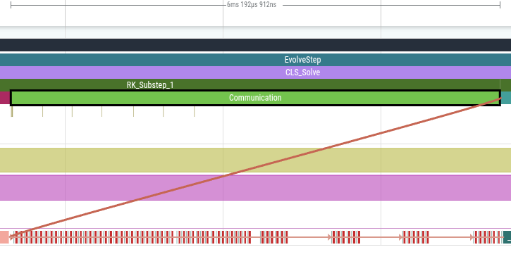
Figure 3: Multiple pack and unpack kernels seen under the “Communication” ROCTx region that took around 6.2ms.

Identifying Bottlenecks with rocprof-compute

With the baseline established, we can now identify specific bottlenecks using more detailed profiling techniques. To understand kernel performance characteristics, we use rocprof-compute for roofline analysis:

rocprof-compute profile -n genasis -- \
  mpirun -np 1 GenASiS_Basics/install/bin/RiemannProblem_rocm-afar \
  Verbosity=INFO_2 nCells=468,468,468 Dimensionality=3D FinishCycle=5

rocprof-compute analyze -p workloads/genasis/mi300a/ -b 4 

Once the profile collection is complete, the rocprof-compute analyze command above will produce roofline information, such as GFLOPs, measured HBM bandwidth, and arithmetic intensity, in Tables 4.1 and 4.2. It is recommended to redirect the output to a file for easier viewing. The kernels will be displayed in order based on percentage of GPU time (shown in parentheticals next to the kernel name). A selection of metrics from the top kernel in this profile are shown below:

Kernel 0: __omp_offloading_38_206d2d__QMpolytropicfluid_formPcomputeeigenspeedskernel_l166 (12.5%)
  |
  ├─ 4.1 Roofline Rate Metrics:
  |   ╒═════════════╤════════════════════╤══════════╤═════════╤════════════════════╕
  |   │ Metric_ID   │ Metric             │    Value │ Unit    │   Peak (Empirical) │
  |   ╞═════════════╪════════════════════╪══════════╪═════════╪════════════════════╡
  |   │ 4.1.1       │ VALU FLOPs (F32)   │     0.16 │ Gflop/s │           96063.54 │
  |   ├─────────────┼────────────────────┼──────────┼─────────┼────────────────────┤
  |   │ 4.1.2       │ VALU FLOPs (F64)   │   212.89 │ Gflop/s │           79287.40 │
  |   ├─────────────┼────────────────────┼──────────┼─────────┼────────────────────┤
  |   │    ...      │         ...        │    ...   │   ...   │         ...        │
  |   ├─────────────┼────────────────────┼──────────┼─────────┼────────────────────┤
  |   │ 4.1.9       │ HBM Bandwidth      │  2844.45 │ Gb/s    │            3343.63 │
  |   ├─────────────┼────────────────────┼──────────┼─────────┼────────────────────┤
  |   │ 4.1.10      │ L2 Cache Bandwidth │  2696.50 │ Gb/s    │           19341.46 │
  |   ├─────────────┼────────────────────┼──────────┼─────────┼────────────────────┤
  |   │ 4.1.11      │ L1 Cache Bandwidth │ 10218.53 │ Gb/s    │           25368.46 │
  |   ├─────────────┼────────────────────┼──────────┼─────────┼────────────────────┤
  |   │ 4.1.12      │ LDS Bandwidth      │     0.95 │ Gb/s    │           57333.99 │
  |   ╘═════════════╧════════════════════╧══════════╧═════════╧════════════════════╛
  ├─ 4.2 Roofline AI Plot Points:
  |   ╒═════════════╤══════════════════════╤═════════╤════════════╕
  |   │ Metric_ID   │ Metric               │   Value │ Unit       │
  |   ╞═════════════╪══════════════════════╪═════════╪════════════╡
  |   │ 4.2.0       │ AI HBM               │    0.07 │ Flops/byte │
  |   ├─────────────┼──────────────────────┼─────────┼────────────┤
  |   │ 4.2.1       │ AI L2                │    0.08 │ Flops/byte │
  |   ├─────────────┼──────────────────────┼─────────┼────────────┤
  |   │ 4.2.2       │ AI L1                │    0.02 │ Flops/byte │
  |   ├─────────────┼──────────────────────┼─────────┼────────────┤
  |   │ 4.2.3       │ Performance (GFLOPs) │  213.02 │ Gflop/s    │
  |   ╘═════════════╧══════════════════════╧═════════╧════════════╛

Note that the rocprof-compute analyze command will also generate a CLI roofline plot. For each kernel in the analyze output, we can see the measured HBM Bandwidth (4.1.9) and compare it with the empirical peak for the device. The arithmetic intensity (4.2.0) tells us whether we are in the bandwidth-bound or compute-bound regime. The table below is a summary of the top 10 kernels:

Kernel	% GPU Time	AI (HBM)	HBM BW (GB/s)	% Peak BW
computeeigenspeedskernel_l166	12.5%	0.07	2844	85%
computefluxeskernel_l225	10.6%	0.35	2868	86%
computefluxeskernel_l290	10.5%	0.35	2880	86%
computeconservedkernel_l19 (pressureless)	8.3%	0.05	3149	94%
computeauxiliarykernel_l104	8.3%	4.53	2137	64%
computereconstructionkernel_l156	8.0%	0.25	3063	92%
computeconservedkernel_l19 (polytropic)	6.5%	0.17	3023	90%
computerawfluxeskernel_l280	6.3%	0.13	3101	93%
computeupdatekernel_l358	5.2%	0.09	3128	94%
computeeigenspeedskernel_l155	5.1%	1.00	2782	83%

Given the relatively low arithmetic intensity for all the top kernels, this confirms that GenASiS kernels are memory-bound; the top kernels are currently measuring at 64-94% of peak empirical bandwidth[1].

Multi-Device Profiling

Profiling MPI applications running on multiple GPUs is not very different from profiling a single-process run. We will first see how to collect timeline traces for multi-process runs and then proceed to answer questions such as:

• Is there any load imbalance when running on multiple GPUs? (see Load Imbalance Analysis section)

• What is the communication overhead when we run multiple processes? (see Communication Overhead Analysis section)

For proper baseline measurement in a multi-process run, ensure proper GPU and CPU core affinity settings such that each process uses a different GPU device. Setting proper affinity on other systems could be challenging. The ROCm blog posts Affinity Part 1 and Affinity Part 2 can help you understand your system’s topology and set up affinity accordingly.

Collecting a Timeline Trace for a Multi-Process Run

To generate a trace of this multi-process run, we simply run rocprofv3 --runtime-trace with the %rank% qualifier in the output filename so that the profiling tool automatically generates separate profiles for each MPI rank (e.g., trace_0_results.db, trace_1_results.db). Note that while rocprofv3 can trace GPU and host-side runtime (HIP, HSA, ROCTx) activity in multi-process MPI applications, it does not trace MPI calls. To trace MPI communications and study network performance, use the ROCm Systems Profiler as described in our previous article in the profiling guide series.

mpirun -np 4 \
  rocprofv3 --runtime-trace -o trace_%rank% -d outdir -- \
  ./GenASiS_Basics/install/bin/RiemannProblem_rocm-afar \
  Verbosity=INFO_2 nCells=468,468,468 Dimensionality=3D FinishCycle=5 \
  nBricks=4,1,1

Even though affinity setup is not shown in the above command, it is highly recommended with each run. On Frontier-style systems, --gpu-bind=closest with one GPU per task is typical.

rocpd can then be used to generate a combined profile with timelines for each rank merged into one Perfetto trace file.

rocpd2pftrace -i outdir/trace_*_results.db -d outdir -o merged

The merged trace in outdir/merged_results.pftrace can then be visualized in the Perfetto UI.

Load Imbalance Analysis

Timeline traces can help you spot load imbalance, if any, between MPI ranks. For instance, the command shown above running with a (4,1,1) 1D process grid produces a timeline trace such as the one shown in Figure 4.

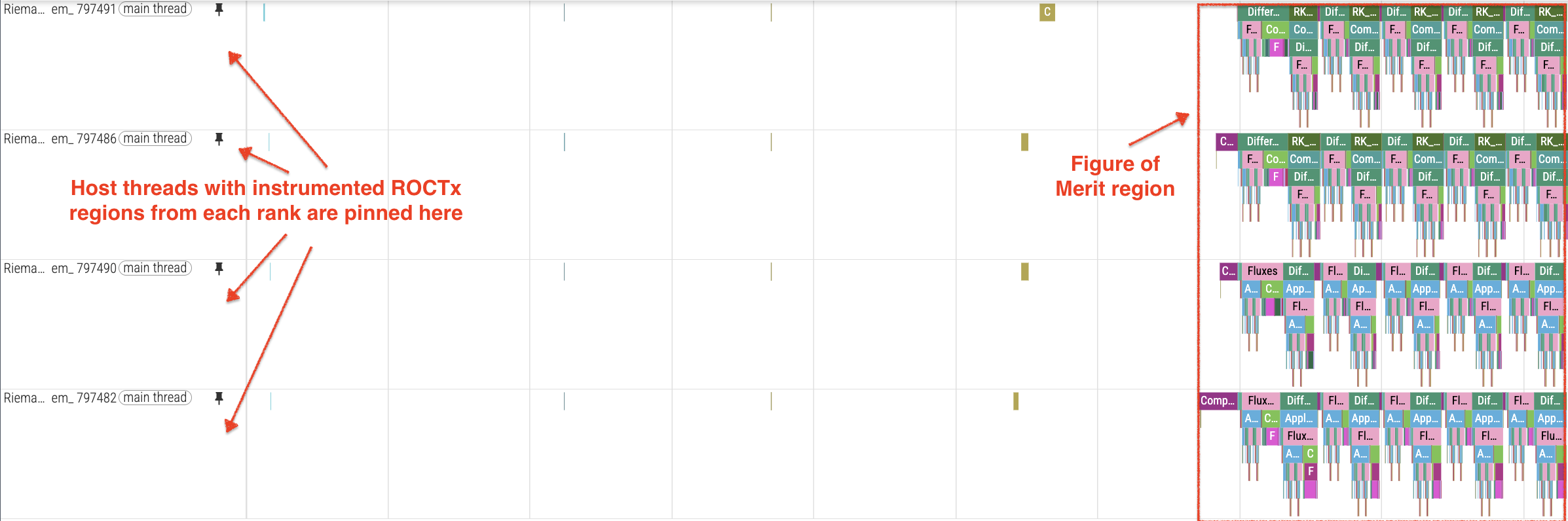
Figure 4: Snapshot from a multi-device trace (4,1,1) showing the activity of 4 MPI ranks arranged in a 1D process grid.

Zooming in to the start of the FoM region as seen in Figure 5, we see vastly different durations of the initial ComputeTimeStep region between the various ranks. This could be explained by first-touch penalties as described in the HSA_XNACK Tuning section.

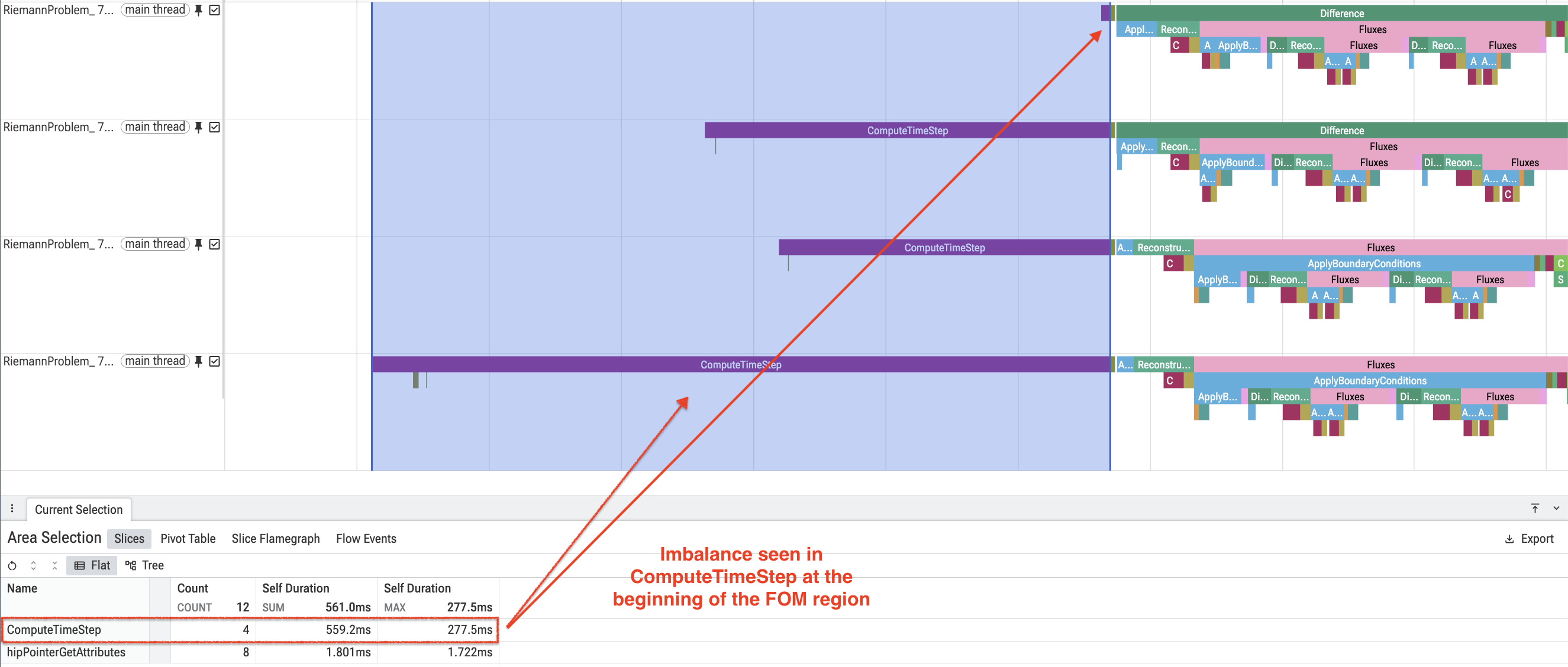
Figure 5: Snapshot of the start of the FoM region in multi-device trace (4,1,1) showing imbalance in ComputeTimeStep region.

Focusing on the activity that follows in the various timesteps as shown in Figure 6, we observe that although specific regions such as ApplyBoundaryConditions show uneven durations, the elapsed time for each timestep is pretty even across the 4 ranks.

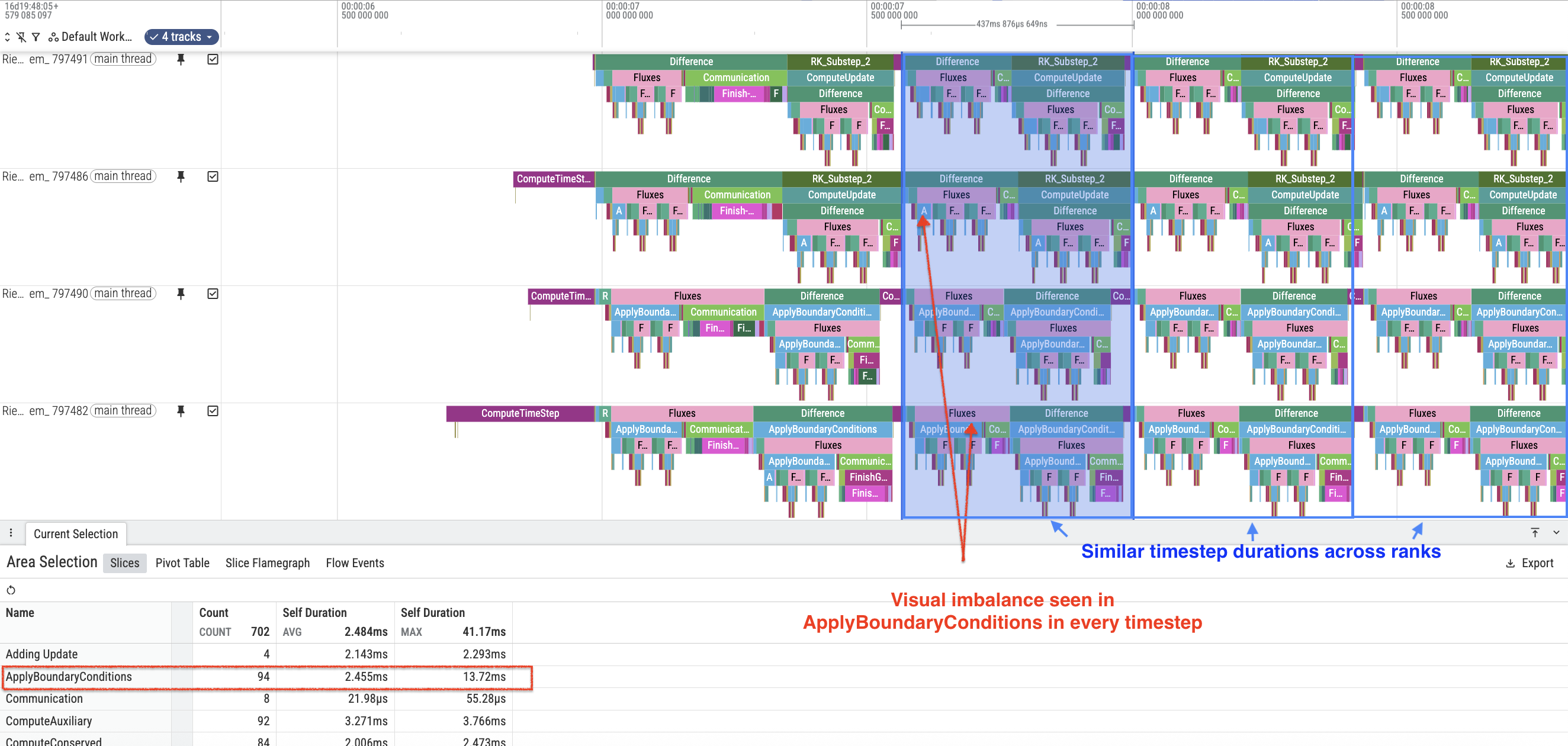
Figure 6: Snapshot of the other timesteps in the FoM region in multi-device trace (4,1,1) showing imbalance in ApplyBoundaryConditions region.

This leads us to conclude that there is no obvious load imbalance in this run of GenASiS.

Communication Overhead Analysis

Analysis of GenASiS timing data shows that computation dominates runtime, with the computation-to-communication ratio ranging from 4x to 6x[1] depending on problem size and rank configuration. Larger problems show better computation-to-communication ratios because the communication overhead (ghost cell exchanges) grows with surface area while computation grows with volume. GenASiS uses GPU-direct communication (DevicesCommunicate = TRUE), eliminating host-device transfers during message passing.

Configuration	Computation	Communication	Ratio
4-rank, 256 × 256 × 256 grid	1.59 s	0.37 s	4.3x
16-rank, 512 × 512 × 512 grid (4,4,1)	3.75 s	0.65 s	5.8x
16-rank, 1024 × 512 × 512 grid	5.08 s	0.78 s	6.5x

However, zooming in to just the Communication region across ranks as shown in Figure 7, we see visual staggering of communication regions across ranks that may need further investigation. At the scales shown here, computation still dominates overall runtime, but the rank-to-rank variation in the Communication region may be worth revisiting at higher node counts, where network effects and synchronization costs may become more pronounced.

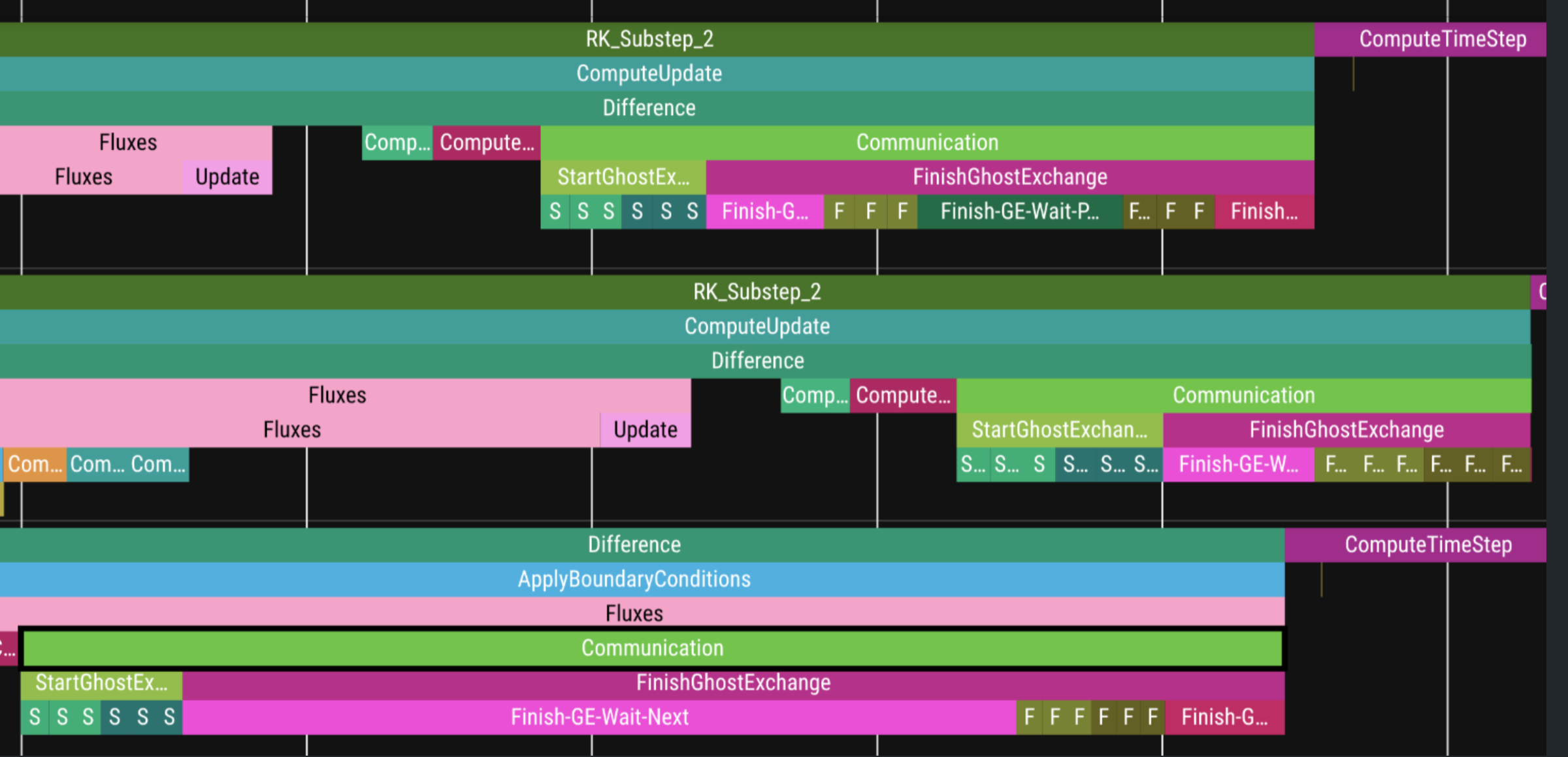
Figure 7: Some differences in the “Communication” ROCTx region between ranks.

Perform Optimizations

Based on our analysis of profiles collected so far, we can apply targeted optimizations. We demonstrate two techniques and summarize the outcome:

1. HSA_XNACK for Production: Enable HSA_XNACK=1 for longer runs, as it may bring performance benefits after initial page migration (see HSA_XNACK Tuning section).

2. Workgroup Size Tuning: Due to the flat nature of the profile, tune and find the optimal workgroup size for each kernel (see Workgroup Size Tuning with thread_limit section).

HSA_XNACK Tuning

The HSA_XNACK environment variable is specific to AMD devices that support a unified memory programming model, such as MI300A, where the CPU and GPU share the same physical address space. Specifically, the HSA_XNACK variable controls page migration behavior for the unified memory model. For a detailed explanation, see the documentation on ROCm ROCR Runtime environment variables and Unified memory management.

GenASiS performance is sensitive to this setting:

• HSA_XNACK=0 (discrete GPU mode): Recommended for profiling short runs (3-5 cycles) to avoid first-touch penalties that skew kernel statistics.

• HSA_XNACK=1 (unified memory mode): Can provide better performance for longer production runs once page migration completes.

Several factors contribute to this performance difference. One is how OpenMP map(to:) and map(tofrom:) clauses are implemented in each setting. With HSA_XNACK=0, these clauses trigger explicit host-to-device copies. With HSA_XNACK=1, the runtime instead registers the host pointer for direct GPU access; the device reads host memory on demand via page faults (XNACK), so no explicit copy occurs. The clause still declares the mapping and triggers setup—it is not a no-op—but the implementation switches from allocate-and-copy to zero-copy shared memory access. These details can be inspected via the LIBOMPTARGET_INFO, LIBOMPTARGET_DEBUG, and AMD_LOG_LEVEL environment variables.

Setting	map(to:) behavior	Data transfer cost
HSA_XNACK=1	No explicit copy; GPU accesses host memory directly	0 s (zero-copy)
HSA_XNACK=0	Explicit host→device copy	Non-zero transfer time

When comparing kernel performance with and without HSA_XNACK, we observed significant differences. For example, comparing second dispatches of the top kernels (after first-touch penalty):

Kernel	XNACK=1	XNACK=0	Perf Delta
computefluxeskernel_l225	0.84 ms	2.05 ms	-59%
computefluxeskernel_l290	0.84 ms	2.05 ms	-59%
computereconstructionkernel_l156	1.23 ms	1.28 ms	-4%
computeconservedkernel_l19	1.73 ms	1.78 ms	-2%
computeupdatekernel_l358	0.98 ms	1.00 ms	-2%

This demonstrates that HSA_XNACK=1 can provide up to 59% better kernel performance[1] for some kernels once page migration completes.

The traces in Figure 8 and Figure 9 illustrate the difference in memory transfer behavior, showing the MEMORY_COPY instances in a 5-cycle run:

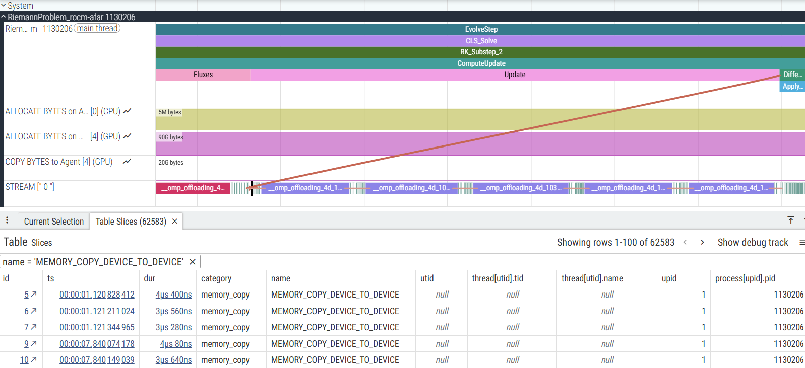
Figure 8: Perfetto trace with HSA_XNACK=0 showing 62,583 MEMORY_COPY instances.

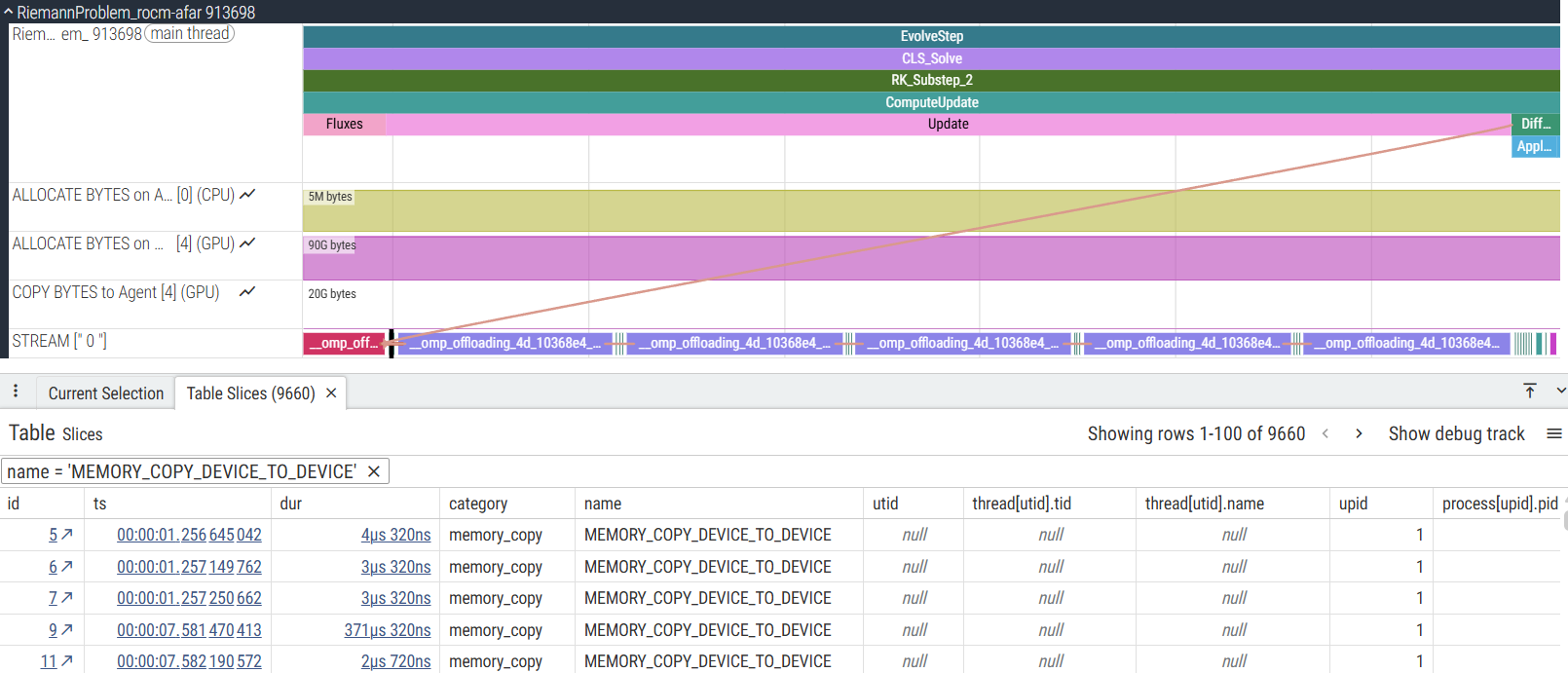
Figure 9: Perfetto trace with HSA_XNACK=1 showing only 9,660 MEMORY_COPY instances (84% reduction)[1].

Workgroup Size Tuning with thread_limit

Since computation dominates communication (as shown in the previous section), we prioritize compute kernel optimizations first. Specifically, we explore workgroup size tuning as a candidate optimization across the top kernels.

In the OpenMP programming model, a team maps naturally to a GPU workgroup, and thread_limit controls the maximum number of OpenMP threads in each team. Adjusting thread_limit can change the GPU workgroup size, which can affect occupancy, latency hiding, and scheduling overhead, making it a useful parameter to test when tuning kernel performance.

The following example, based on the computeeigenspeedskernel from GenASiS (PolytropicFluid_Kernel.f90), shows how thread_limit can be added to a target directive:

Default (256 threads per team)

With thread_limit(512)

!$OMP target teams distribute & !$OMP parallel do simd schedule ( auto ) do iV = 1, size ( N ) FEP_1 ( iV ) = V_1 ( iV ) + CS ( iV ) FEP_2 ( iV ) = V_2 ( iV ) + CS ( iV ) FEP_3 ( iV ) = V_3 ( iV ) + CS ( iV ) FEM_1 ( iV ) = V_1 ( iV ) - CS ( iV ) FEM_2 ( iV ) = V_2 ( iV ) - CS ( iV ) FEM_3 ( iV ) = V_3 ( iV ) - CS ( iV ) end do !$OMP end target teams distribute & !$OMP parallel do simd

!$OMP target teams distribute & !$OMP parallel do simd schedule ( auto ) & !$OMP thread_limit(512) do iV = 1, size ( N ) FEP_1 ( iV ) = V_1 ( iV ) + CS ( iV ) FEP_2 ( iV ) = V_2 ( iV ) + CS ( iV ) FEP_3 ( iV ) = V_3 ( iV ) + CS ( iV ) FEM_1 ( iV ) = V_1 ( iV ) - CS ( iV ) FEM_2 ( iV ) = V_2 ( iV ) - CS ( iV ) FEM_3 ( iV ) = V_3 ( iV ) - CS ( iV ) end do !$OMP end target teams distribute & !$OMP parallel do simd

Note: GenASiS uses preprocessor macros (e.g., OMP_TARGET_DIRECTIVE) to abstract the target directives. The above shows the expanded form when compiled with OpenMP target offload enabled.

We explored different workgroup sizes on the top hotspot kernel, computeeigenspeedskernel_l166. The performance comparison shown in the table below is also plotted in Figure 10.

Workgroup Size	Teams	Avg Time (ms)	Performance vs Default
64	3648	3.17	+5.7% slower
128	1824	3.19	+6.3% slower
256 (default)	912	3.00	(reference)
512	456	2.92	-2.7% (Best)
1024	456	3.42	+14.0% (Worst)

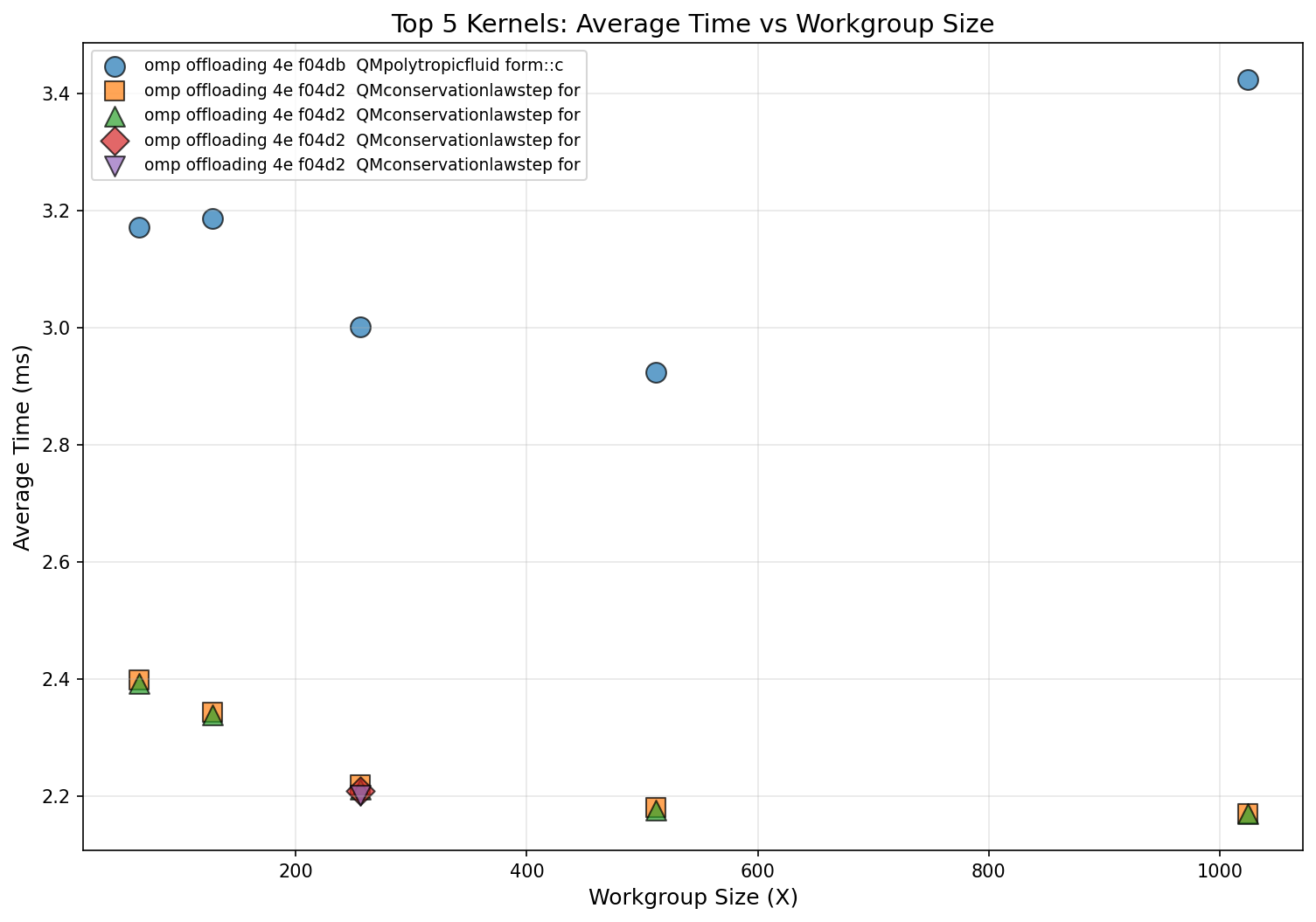
Figure 10: Workgroup size performance trends across top kernels.

The optimal workgroup size for this kernel is 512 threads, providing approximately 3% improvement[1] over the default (256 threads) and 17% faster[1] than the worst configuration (1024 threads). However, applying this optimization uniformly showed minimal impact on overall execution time because the kernel accounts for only ~12% of total GPU time. As expected from the flat profile identified in the kernel hotspot analysis, per-kernel tuning yields incremental rather than transformative gains.

Potential future optimizations that could provide larger impact include:

• Bundling communication operations to reduce message overhead (currently 72 pack/unpack kernels per communication phase).

• Addressing the load imbalance in ApplyBoundaryConditions observed in multi-device runs.

• Exploring GPU oversubscription (running multiple MPI ranks per GPU) to better utilize GPU resources since AMD GPUs natively allow oversubscription and require no special additional setup.

Summary

In the previous profiling guide series blog posts (Part 1, Part 2, and Part 3), we explored the profiling process using AMD tools with single-process and multi-process GPU applications. This post delves into using the same tools specifically for Fortran OpenMP offload applications, with an additional focus on profiling techniques tailored for Fortran codebases. Beyond identifying GPU kernel bottlenecks, we also analyzed host-side performance and data movement patterns that can help unlock optimization opportunities for Fortran applications. In this blog post, we also benefited from the “profile once, analyze many times” workflow using rocpd.

Through the GenASiS example, we demonstrated:

1. Establishing Baselines: Identifying appropriate problem size (468 × 468 × 468 per device) and HSA_XNACK settings for profiling vs. production.

2. Identifying Bottlenecks: rocprofv3 kernel traces revealed a flat profile, while timeline traces showed imbalance in some ROCTx regions.

3. Deep Kernel Analysis: rocprof-compute roofline analysis confirmed bandwidth-limited kernels operating at 64-94% of peak bandwidth, indicating memory-bound behavior.

4. Multi-Device Analysis: Timeline traces for multi-process runs revealed minor load imbalance patterns; communication overhead analysis showed a 4-6x computation-to-communication ratio that improves with problem size, leading to prioritization of compute kernel optimization.

5. HSA_XNACK Impact: Enabling XNACK can improve kernel performance (up to 59% for some kernels) but introduces first-touch penalties that skew short-run statistics.

6. Workgroup Tuning: Exploring thread_limit settings showed 512 threads optimal for the top kernel (~3% improvement over the default 256), though overall application impact was limited due to the flat profile.

The small gains seen here are consistent with a flat, memory-bound application; the profiling process correctly identified that no single optimization would be transformative. The real takeaway is the workflow itself: establish baselines, collect targeted profiles, interpret the data, and iterate. Apply the same approaches to your own Fortran OpenMP offload application to understand how well it is utilizing the available hardware and where further optimization opportunities lie.

Useful Resources

• Performance Profiling on AMD GPUs Blog Posts:

  • Part 1

  • Part 2

  • Part 3

• Perfetto UI:

  • Online documentation for using Perfetto UI

• rocprofiler-sdk:

  • Open source at rocprofiler-sdk github repo

  • rocprofiler-sdk documentation

  • rocprofv3 documentation

  • rocpd documentation

• rocprof-sys:

  • Open source at rocprofiler-systems github repo

  • ROCm Systems Profiler documentation

• rocprof-compute:

  • Open source at rocprofiler-compute github repo

  • ROCm Compute Profiler documentation

• hipfort:

  • Open source at hipfort github repo

  • hipfort documentation

• AMD Fortran Compiler (amdflang):

  • Introducing AMD’s Next-Gen Fortran Compiler

  • ROCm AFAR pre-production builds

Disclaimers

The information presented in this document is for informational purposes only and may contain technical inaccuracies, omissions, and typographical errors. The information contained herein is subject to change and may be rendered inaccurate for many reasons, including but not limited to product and roadmap changes, component and motherboard version changes, new model and/or product releases, product differences between differing manufacturers, software changes, BIOS flashes, firmware upgrades, or the like. Any computer system has risks of security vulnerabilities that cannot be completely prevented or mitigated. AMD assumes no obligation to update or otherwise correct or revise this information. However, AMD reserves the right to revise this information and to make changes from time to time to the content hereof without obligation of AMD to notify any person of such revisions or changes. THIS INFORMATION IS PROVIDED ‘AS IS.” AMD MAKES NO REPRESENTATIONS OR WARRANTIES WITH RESPECT TO THE CONTENTS HEREOF AND ASSUMES NO RESPONSIBILITY FOR ANY INACCURACIES, ERRORS, OR OMISSIONS THAT MAY APPEAR IN THIS INFORMATION. AMD SPECIFICALLY DISCLAIMS ANY IMPLIED WARRANTIES OF NON-INFRINGEMENT, MERCHANTABILITY, OR FITNESS FOR ANY PARTICULAR PURPOSE. IN NO EVENT WILL AMD BE LIABLE TO ANY PERSON FOR ANY RELIANCE, DIRECT, INDIRECT, SPECIAL, OR OTHER CONSEQUENTIAL DAMAGES ARISING FROM THE USE OF ANY INFORMATION CONTAINED HEREIN, EVEN IF AMD IS EXPRESSLY ADVISED OF THE POSSIBILITY OF SUCH DAMAGES. AMD, the AMD Arrow logo, and combinations thereof are trademarks of Advanced Micro Devices, Inc. Other product names used in this publication are for identification purposes only and may be trademarks of their respective companies. © 2026 Advanced Micro Devices, Inc. All rights reserved

---

[1] (1,2,3,4,5,6,7)

Based on AMD internal testing in Q4 2025 and Q1 2026, measuring kernel execution time and other performance characteristics of the GenASiS_Basics RiemannProblem benchmark on a test system configured with an HPE Cray EX255a blade containing 4x AMD Instinct™ MI300A APUs (4x 128 GB HBM3 memory, 96 integrated AMD EPYC™ “Zen 4” CPU cores), and AMD ROCm™ 7.2 software. GenASiS was compiled with amdflang from the ROCm AFAR drop 22.2.0 toolchain. System manufacturers may vary in configurations, yielding different results. Performance may vary based on the use of the latest drivers and optimizations.