Scaling 3D Gaussian Splatting with Distributed Compute: Why One GPU Is Never Enough

October 23, 2026 by Ish Kool, Shaghayegh Roohi, Mark Granroth Wilding, Deeksha Goplani, Karthik Kashyap Thatipamula, Pier Luigi Dovesi, Vish Vadlamani, Vikas C Sajjan, Phani Vaddadi..

22 min read. | 5488 total words.

Software tools & optimizations

AI/ML, HPC, Computer Vision, Memory, Performance, PyTorch

Developers

gsplat is a GPU-optimized Python library for training and rendering 3D Gaussian Splatting (3DGS) models. In earlier posts we showed how to train gsplat scenes on AMD GPUs, took a closer look at the mathematics of 3DGS, and applied gsplat to autonomous driving.

All of those examples fit comfortably on one GPU. Real production scenes do not. A city block captured at 4K resolution needs tens of millions of Gaussians, and the parameters plus optimizer state alone will exhaust the memory of any single accelerator long before reconstruction quality stops improving.

This post explains why that wall appears so quickly, what distributed training does about it, and precisely how gsplat implements it on AMD Instinct™ GPUs. Along the way we walk through the parallelization strategy collective call by collective call, because gsplat’s approach is a genuinely unusual one: it is data-parallel in spirit, but it never once all-reduces a gradient of the scene it is training. We then check that walkthrough against a rocprofv3 trace of a real four-GPU run, which both confirms the design and shows that the obvious suspect for a bottleneck is not the guilty one.

Where the Memory Goes

3DGS represents a scene as a set of anisotropic Gaussians rather than voxels or meshes. Each Gaussian is parameterized by:

• The mean \(\mu \in \mathbb{R}^3\), the position of the Gaussian’s center.

• The covariance matrix \(\Sigma \in \mathbb{R}^{3 \times 3}\), which defines the Gaussian’s shape and orientation.

• The color \(c\), encoded as spherical harmonics (SH) coefficients.

• The opacity \(\alpha \in [0,1]\).

Assuming float32 (4 bytes per scalar), a single Gaussian primitive costs:

Component	Parameters	Bytes
Mean \((x, y, z)\)	3	12
Covariance: scale \(\mathbf{s} \in \mathbb{R}^3\) + quaternion \(q \in \mathbb{R}^4\)	7	28
View-dependent color: 9 SH coefficients per channel (degree 2)	27	108
Opacity	1	4
Learnable subtotal	38	152
Adam optimizer state (first and second moments)	76	304
Total	114	456

At 456 bytes per primitive, the arithmetic is unforgiving:

• 1M Gaussians requires 456 MB

• 100M Gaussians requires 45 GB

• 1B Gaussians requires 456 GB

Two things make the real picture worse. First, this accounting assumes SH degree 2, whereas gsplat’s simple_trainer.py defaults to sh_degree=3, which means 16 coefficients per channel instead of 9. That raises the learnable parameter count from 38 to 59 and the total cost with Adam state to roughly 708 bytes per Gaussian. Second, none of this includes the transient cost of a training step: the gradient buffers, the projected 2D means and conics, and above all the per-tile sorted lists of Gaussian-to-pixel intersections. Those intersection buffers scale with image resolution and Gaussian density, and at 4K they are frequently what actually triggers an out-of-memory error.

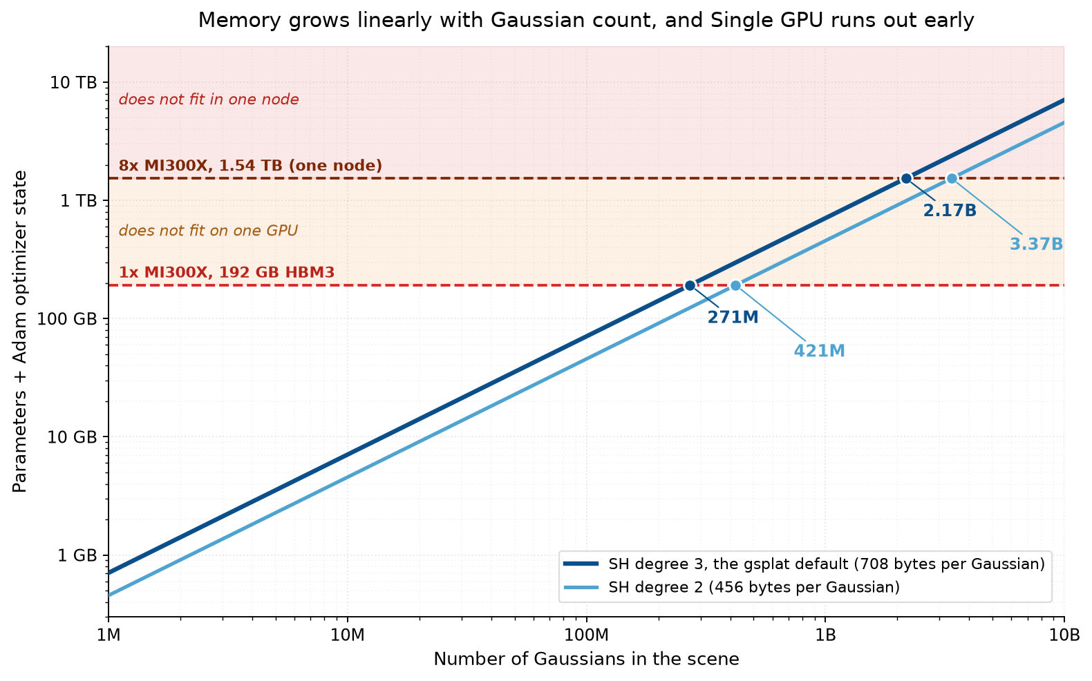
Figure 1: Memory for parameters and optimizer state grows linearly with the number of Gaussians. A single MI300X with 192 GB of HBM3 runs out at 271 million Gaussians at gsplat’s default SH degree 3, or 421 million at SH degree 2. A full eight-GPU node moves that ceiling to 2.17 billion. Gradient buffers and the per-tile intersection lists are excluded, so in practice you hit an out-of-memory error before reaching these lines.

Why More VRAM Alone Does Not Solve It

A natural reaction to Figure 1 is to ask for a bigger GPU. That helps, but it addresses only one of the three limits you hit:

• Throughput does not scale with capacity. Training speed is bounded by compute-unit count and memory bandwidth. Doubling HBM capacity adds neither. A scene that fits but trains for a week is not a usable scene.

• Quality is capped by whatever fits. When memory is the constraint, the only lever is to densify less aggressively and prune harder, which directly removes the fine detail that motivated the large capture in the first place.

• Rendering latency is bounded by one memory bus. A single device must stream every visible Gaussian for every frame through one memory hierarchy.

Distributing the work attacks all three at once. It gives you feasibility (the scene fits), quality (you can keep the Gaussians densification produces), and throughput (more compute units working per unit time).

A Short Primer on Distributed Training

Before looking at what gsplat does, it is worth being precise about what distributed training normally means, because gsplat keeps some of the standard machinery and discards the rest.

What Consumes Memory in a Training Step

Any gradient-based training job spends memory on four things:

1. Parameters — the values being optimized.

2. Gradients — one value per parameter, produced by the backward pass.

3. Optimizer state — for Adam, two moments per parameter, so 2x the parameter footprint.

4. Activations — intermediate tensors saved by the forward pass so the backward pass can use them.

In a large language model, parameters and optimizer state dominate and activations are a tunable fraction you can trade against recomputation. In 3DGS the balance is different: the parameters are the scene, so they grow as reconstruction quality improves, and the dominant “activation” is the per-pixel list of intersecting Gaussians, whose size depends on scene content rather than on a fixed architecture.

Data Parallelism and PyTorch DDP

The most widely used parallelization strategy is data parallelism, implemented in PyTorch as DistributedDataParallel (DDP). One process is launched per GPU, and each process:

1. Holds a complete replica of the model parameters and optimizer state.

2. Receives a different slice of the input batch.

3. Runs forward and backward locally, producing gradients that differ across ranks because the data differed.

4. All-reduces the gradients so every rank ends up with the mean gradient over the global batch.

5. Applies an identical optimizer step, which keeps the replicas bit-identical.

DDP overlaps step 4 with step 3 by grouping parameters into buckets and firing an asynchronous all-reduce as soon as each bucket’s gradients are ready, so communication hides behind the remaining backward computation.

The critical property of DDP is that it scales throughput, not capacity. Every rank still stores the whole model, so DDP alone can never train a model that does not fit on one GPU. Techniques that shard parameters and optimizer state, such as FSDP and ZeRO, exist precisely to lift that restriction. As we will see, gsplat needs the capacity benefit, so plain DDP over the Gaussians was never an option.

RCCL: The Transport Layer

Those all-reduces have to physically move bytes between GPUs. On AMD hardware that job belongs to RCCL, the ROCm Communication Collectives Library. RCCL is API-compatible with NVIDIA’s NCCL, which is why you still write backend="nccl" in PyTorch on ROCm and why every tuning knob is still spelled NCCL_*:

torch.distributed.init_process_group(
    backend="nccl", world_size=world_size, rank=world_rank
)

RCCL implements the collectives that distributed training depends on:

Collective	What it does	Typical use
all_reduce	Combines a tensor from every rank and returns the result to every rank	Gradient averaging in DDP
all_gather	Concatenates each rank’s tensor on every rank	Collecting shard metadata; FSDP weight gathering
reduce_scatter	Combines tensors, then gives each rank one slice of the result	Backward pass of a differentiable all_gather
broadcast	Copies one rank’s tensor to all ranks	Initial state synchronization
all_to_all	Each rank sends a distinct payload to every other rank	Expert routing in MoE; Gaussian exchange in gsplat

all_reduce is not a primitive. RCCL implements it in the ring algorithm as a reduce-scatter followed by an all-gather, each of which moves \(\frac{n-1}{n}\) of the buffer around a logical ring of \(n\) ranks. That decomposition is visible in any collective trace and is worth recognizing, because a single logical all_reduce in your Python code shows up as two distinct communication phases on the wire.

On an AMD Instinct MI300X node the ring is mapped onto xGMI links, where all eight GPUs are directly connected to one another. Each link is rated at 64 GB/s per direction with roughly 45-48 GB/s achievable after protocol overhead. Two practical consequences follow. First, collectives are fastest when all eight GPUs participate, since every link is then active. Second, when you deliberately run on 2 or 4 GPUs, most of the node’s aggregate link bandwidth sits idle; NCCL_MIN_NCHANNELS can recover some of it by increasing the number of channels RCCL uses.

Why gsplat Cannot Just Use DDP

3DGS training is gradient descent, so everything you know about gradient descent still applies. The objective is a weighted combination of an L1 term and a D-SSIM term between the rendered image and the ground truth:

\[ \mathcal{L} = (1 - \lambda) \left( \frac{1}{N} \sum_{i=1}^{N} \left| I_{\text{r}}(i) - I_{\text{gt}}(i) \right| \right) + \lambda \left( \frac{1 - \text{SSIM}(I_{\text{r}}, I_{\text{gt}})}{2} \right) \]

where \(I_{\text{r}}\) is the rendered image, \(I_{\text{gt}}\) the ground truth, \(N\) the pixel count, and \(\lambda\) balances the two terms. Gradients flow back to \(\mu\), \(\Sigma\), \(c\), and \(\alpha\) exactly as they would flow back to the weights of a network.

The similarity ends there, and the differences are what rule out a straightforward DDP setup:

• The parameters are the data. There is no compact model that generalizes over a dataset; the Gaussians are the reconstruction. Replicating them on every rank, as DDP requires, replicates the very thing that does not fit.

• The parameter count changes during training. Adaptive density control clones, splits, and prunes Gaussians every hundred steps. DDP assumes a static parameter set registered once at construction time.

• Each parameter touches a tiny, view-dependent subset of the output. A Gaussian’s footprint typically covers a small patch of the image, and which patch depends on the camera. There is no dense matrix multiply in which every parameter contributes to every output.

• The workload is inherently unbalanced. A region of sky intersects far fewer Gaussians than a region of foliage, and that distribution shifts as densification proceeds.

The last two points are the interesting ones. Because a Gaussian only matters to the cameras that can see it, gsplat can route the Gaussians a given camera needs to the rank rendering that camera instead of replicating everything everywhere. That is a targeted, directional exchange rather than a symmetric reduction, and it is the reason the dominant collective in gsplat is all_to_all rather than all_reduce.

Here is how the standard data-parallel playbook maps onto gsplat:

DDP concept	Does gsplat use it?
One process per GPU, nccl/RCCL backend	Yes, via gsplat.distributed.cli
Each rank sees different input data	Yes, each rank draws its own camera views
Replicated parameters	No. Each rank owns a disjoint shard of the Gaussians
all_reduce of gradients	No, not for the Gaussians. Gradients reach their owner through the reverse of the forward exchange
Identical optimizer step on every rank	No. Each rank runs Adam over its own shard only
Learning rate scaled for the global batch	Yes, by \(\sqrt{\text{batch size} \times \text{world size}}\)
DDP wrapper on torch.nn.Module	Yes, but only for the small auxiliary modules

The third and fourth rows are the crux, and they are worth stating plainly because the opposite is a common misconception: gsplat never all-reduces the gradients of the Gaussian parameters. There is no gradient averaging over the scene, because there is nothing to average — each Gaussian exists on exactly one rank.

How gsplat Partitions the Work

gsplat exploits the fact that different stages of a training iteration are parallel along different axes:

• Projection transforms each Gaussian into screen space for a given camera. It is per-Gaussian work, so it parallelizes over Gaussians.

• Rasterization and loss compute pixel colors and compare them to ground truth. That is per-pixel work belonging to a specific image, so it parallelizes over cameras.

As shown in the diagram below, gsplat partitions Gaussians for the first stage and cameras for the second, and exchanges data between the two. The axis of parallelism changes in the middle of the iteration, which is why an exchange is needed at all:

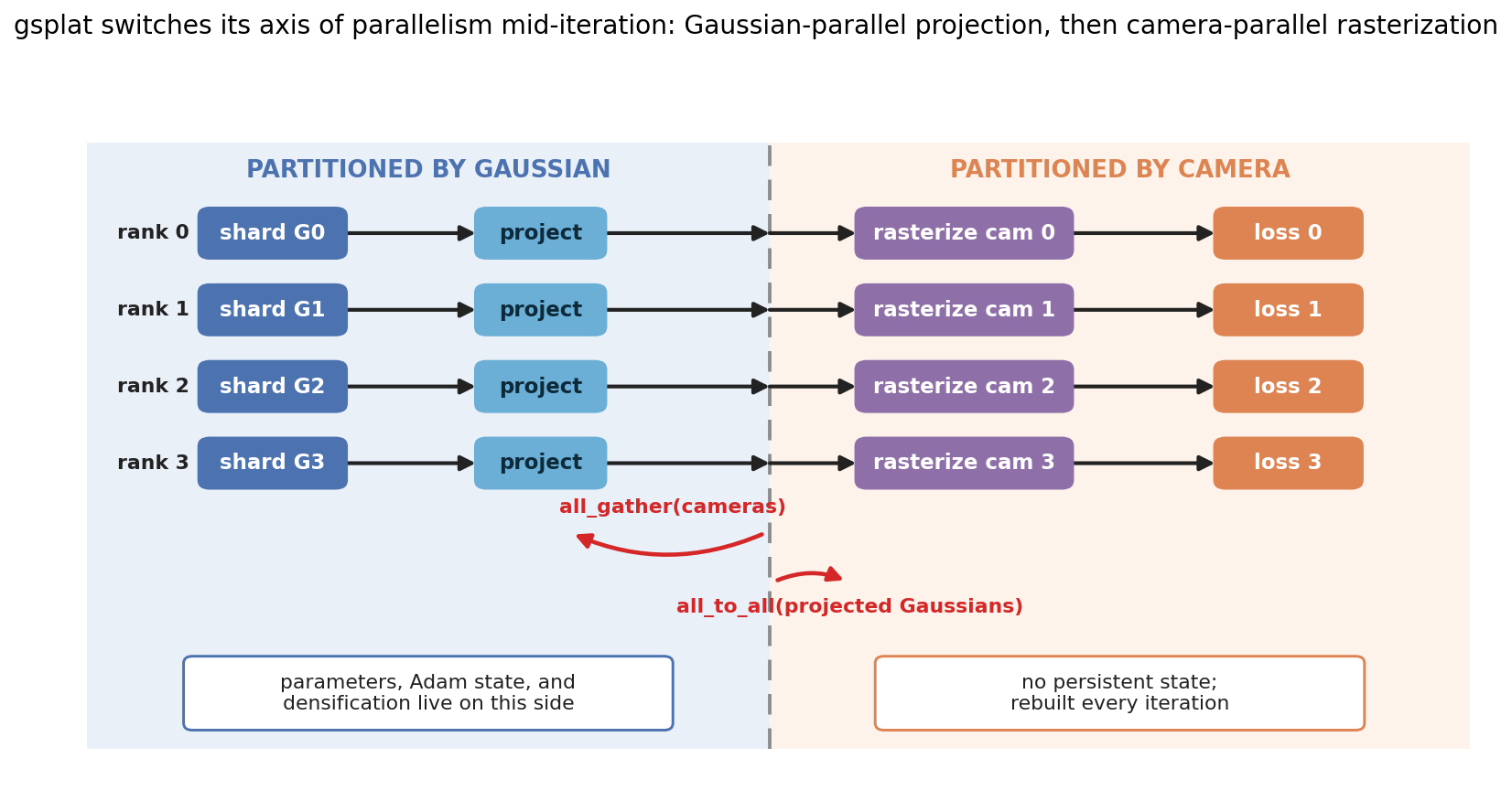
Figure 2: gsplat changes its axis of parallelism in the middle of an iteration. The left half is partitioned by Gaussian, so each rank owns a disjoint shard and projects it; the right half is partitioned by camera, so each rank rasterizes and computes loss for its own views. An all_gather copies the camera set onto every rank before projection, and an all_to_all routes the projected Gaussian records to whichever rank owns the camera that needs them. Parameters, Adam state, and densification live entirely on the Gaussian side; the camera side holds no persistent state and is rebuilt every iteration.

The partition of Gaussians is a plain strided round-robin split performed once at initialization, in create_splats_with_optimizers:

# examples/simple_trainer.py
# Distribute the GSs to different ranks (also works for single rank)
points = points[world_rank::world_size]
rgbs = rgbs[world_rank::world_size]
scales = scales[world_rank::world_size]

Two things are worth noting. This split is not spatial — there is no octree or grid, and adjacent points in the structure-from-motion point cloud deliberately land on different ranks. And it happens before the parameters and optimizer are constructed, which is what makes the memory saving real: rank \(r\) allocates parameters and Adam state for its \(N/\text{world size}\) Gaussians and never sees the others.

The camera partition needs no explicit code. Each rank builds its own DataLoader over the full training set with a different random seed, so at every step the ranks are working on different views. The rasterizer is then told to cooperate:

# examples/simple_trainer.py, Runner.rasterize_splats()
render_colors, render_alphas, info = rasterization(
    means=means,
    quats=quats,
    scales=scales,
    opacities=opacities,
    colors=colors,
    viewmats=torch.linalg.inv(camtoworlds),
    Ks=Ks,
    width=width,
    height=height,
    packed=self.cfg.packed,
    distributed=self.world_size > 1,
    ...
)

The entire distributed strategy is gated on that one distributed flag, implemented in gsplat/rendering.py on top of the communication helpers in gsplat/distributed.py.

Where DDP Actually Appears

PyTorch’s DistributedDataParallel is used in gsplat, but only for the optional auxiliary modules that are small, static, and replicated: the camera pose optimizer, the pose perturbation module used for robustness experiments, and the per-image appearance embedding network.

# examples/simple_trainer.py, Runner.__init__()
if cfg.pose_opt:
    self.pose_adjust = CameraOptModule(len(self.trainset)).to(self.device)
    ...
    if world_size > 1:
        self.pose_adjust = DDP(self.pose_adjust)

if cfg.app_opt:
    self.app_module = AppearanceOptModule(...).to(self.device)
    ...
    if world_size > 1:
        self.app_module = DDP(self.app_module)

These modules hold a few million parameters at most and every rank needs the same copy, so textbook DDP with gradient all-reduce is exactly right for them. If you train with pose_opt and app_opt disabled, which is the default, there is no all_reduce of any learnable parameter anywhere in the training loop.

One Training Iteration, Collective by Collective

Here is what actually happens in a single step of a multi-GPU gsplat run. Assume world_size = 4, with each rank holding \(N_r\) Gaussians and drawing \(C_{\text{local}}\) camera views.

The Forward Pass

1. Agree on shard sizes. Each rank publishes its local Gaussian count so that everyone can later convert between local and global indices. This is a small all_gather of one 32-bit integer per rank, implemented as all_gather_into_tensor rather than all_gather_object because the latter round-trips through CPU pickling:

   # gsplat/rendering.py
   N_world = all_gather_int32(world_size, N, device=device)
   

2. Gather every camera onto every rank. View matrices and intrinsics are tiny, so each rank simply takes a full copy of the global camera set. After this call, C silently changes meaning from “my cameras” to “all cameras”:

   # gsplat/rendering.py
   C_world = [C] * world_size
   viewmats, Ks = all_gather_tensor_list(world_size, [viewmats, Ks])
   C = len(viewmats)
   

3. Project locally, against every camera globally. Each rank projects its own \(N_r\) Gaussians against all \(C_{\text{local}} \times \text{world size}\) cameras in the job, producing 2D means, depths, conics, radii, and a visibility mask. This is the Gaussian-parallel stage, and it involves no communication at all.

4. Evaluate spherical harmonics before communicating. SH coefficients are converted to a per-camera RGB triple while still on the owning rank. This ordering matters for bandwidth: at sh_degree=3 a Gaussian carries 48 SH coefficients (192 bytes), but only the 3 evaluated color channels (12 bytes) ever cross the interconnect.

5. Ship each camera’s Gaussians to the rank that owns that camera. This is the one large transfer in the iteration, and it takes one of two forms depending on the packed flag.

   With packed=True, projection returns a compacted list containing only the (camera, Gaussian) pairs that actually intersect. Each rank therefore knows exactly how many records it owes each peer, exchanges those counts, and then sends only the visible records:

   # gsplat/rendering.py, packed mode
   cnts = torch.bincount(camera_ids, minlength=C)
   cnts = [cuts.sum() for cuts in cnts.split(C_world, dim=0)]
   
   collected_splits = all_to_all_int32(world_size, cnts, device=device)
   (radii,) = all_to_all_tensor_list(
       world_size, [radii], cnts, output_splits=collected_splits
   )
   (means2d, depths, conics, opacities, colors) = all_to_all_tensor_list(
       world_size,
       [means2d, depths, conics, opacities, colors],
       cnts,
       output_splits=collected_splits,
   )
   

   With packed=False, which is the default, projection returns dense [C, N] tensors and the exchange is dense too: rank \(r\) sends its entire local Gaussian set for every camera each peer owns, visible or not, and the split sizes are pure arithmetic rather than a function of visibility:

   # gsplat/rendering.py, non-packed mode
   C = C_world[world_rank]
   (radii,) = all_to_all_tensor_list(
       world_size,
       [radii.flatten(0, 1)],
       splits=[C_i * N for C_i in C_world],
       output_splits=[C * N_i for N_i in N_world],
   )
   

   Either way the record per (camera, Gaussian) pair is about a dozen scalars — two for radii, two for means2d, one for depths, three for conics, one for opacities, three for colors — so roughly 48 bytes, plus 8 bytes of camera_ids and gaussian_ids in packed mode.

   The distinction matters more than it looks. In the default dense path, the bytes rank \(r\) sends per iteration come to roughly \(48 \times N_r \times C_{\text{local}} \times (W - 1)\), where \(W\) is the world size. For 4 ranks holding 2M Gaussians each and one camera per rank, that is a few hundred megabytes per rank, per iteration, in each direction. Switching on --packed replaces \(N_r\) with the number of Gaussians actually visible, which for a typical view is a small fraction of the scene. If you are scaling out and communication looks like your bottleneck, this is the first flag to try.

6. Rebase the indices. camera_ids produced by projection are global and must become local to the receiving rank, while gaussian_ids are local and must become global so the receiver can attribute gradients correctly. gsplat adjusts both with cumulative offsets before shipping them through a second all_to_all. This step exists only in packed mode; the dense path derives indices from tensor shape.

7. Rasterize locally. Each rank now holds every Gaussian record needed for its own \(C_{\text{local}}\) cameras and rasterizes complete images with no further communication.

8. Compute the loss locally. L1 and fused SSIM against the local ground-truth images, plus any depth or regularization terms.

The Backward Pass

9. Gradients flow back through the same exchange, reversed. The helpers in gsplat/distributed.py dispatch to torch.distributed.nn.functional when the input requires grad, which is what makes them differentiable:

   # gsplat/distributed.py, all_to_all_tensor_list()
   if data.requires_grad:
       # differentiable all_to_all
       distF.all_to_all(collected, data.split(splits, dim=0))
   else:
       torch.distributed.all_to_all(collected, list(data.split(splits, dim=0)))
   

   The transpose of an all_to_all is another all_to_all in the opposite direction, so every Gaussian’s gradient contribution is routed back to the rank that owns it. The transpose of the camera all_gather in step 2 is a reduce-scatter: gradients with respect to the view matrices are summed across ranks and each rank keeps the slice for its own cameras, which is what makes pose optimization correct under sharding.

10. All-reduce the auxiliary modules, if enabled. DDP fires its bucketed all_reduce for pose_adjust and app_module here. If those features are off, this step does not exist.

11. Step the optimizer locally. Each rank runs Adam over its own shard. No synchronization, and no requirement that the shards remain the same size.

12. Densify locally. DefaultStrategy.step_post_backward clones, splits, and prunes based on accumulated 2D position gradients, entirely within the rank. Nothing is communicated.

The shape of the communication is quite different from a conventional DDP job. A DDP step is dominated by a handful of large, symmetric all_reduce calls whose volume is fixed by the parameter count and identical every step. A gsplat step is dominated by directional all_to_all traffic whose volume depends on the Gaussian shard sizes, the number of cameras per rank, and — in packed mode — on how much of the scene each camera can currently see. Nothing is reduced; everything is routed.

What a Real 4-GPU Trace Shows

Everything above is what the source code says should happen. This section is what a profiler actually recorded.

The trace was captured with rocprofv3 on a single node with four Instinct GPUs, one rank per GPU, with kernel dispatch and RCCL API tracing enabled and roctx ranges wrapped around the phases of the training loop (rasterize, loss, backward, optimizer, densify). All four ranks were merged into a single Perfetto trace so their timelines share one clock, and sixty iterations were profiled. The rasterizer’s launch geometry puts the images at roughly 1240x824 pixels, which is 155 by 103 tiles of 8 by 8, consistent with --data_factor 4 on a Mip-NeRF 360 scene. Each rank drew one camera per step, and packed was left at its default of False.

A trace is also a surprisingly good way to check facts about an implementation without reading its source. The projection kernel is launched over one thread per (global camera, local Gaussian) pair while the tile-intersection kernel is launched over one thread per (local camera, global Gaussian) pair, and the two launch geometries together pin the shards at 13,569 Gaussians on three ranks and 13,568 on the fourth, for 54,275 in total. That is exactly the \(\lceil N/W \rceil\) / \(\lfloor N/W \rfloor\) split a strided round-robin produces, and it stays constant across all sixty steps because the default refine_start_iter is 500 — densification has not begun.

Five Collectives Per Iteration, and Zero All-Reduces

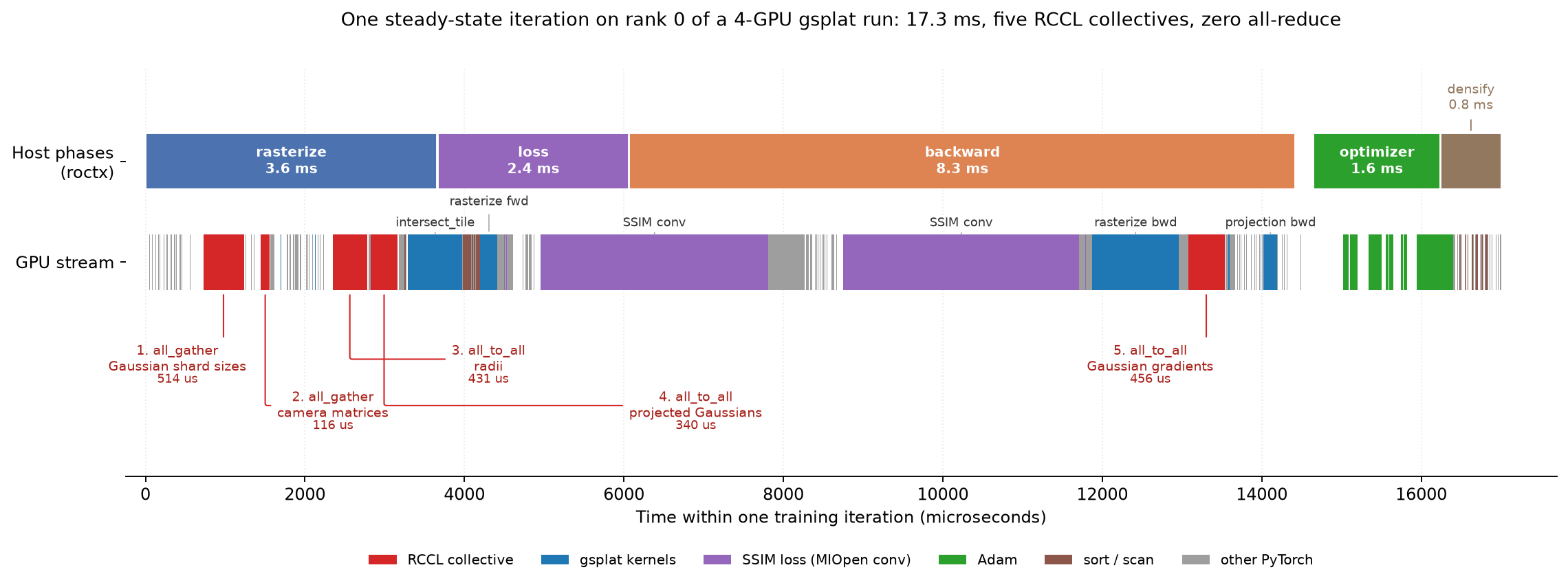
Figure 3: One steady-state iteration on rank 0, reconstructed from the trace. The upper bar is the host-side phase annotation; the lower bar is every kernel that executed on that GPU, colored by category. The five red blocks are the only inter-GPU communication in the step.

Every iteration on every rank has exactly the same communication signature:

#	Collective	RCCL API calls	Host phase	GPU time
1	all_gather of Gaussian shard sizes	1x ncclAllGather	rasterize	0.51 ms
2	all_gather of view matrices and intrinsics	1x ncclAllGather	rasterize	0.12 ms
3	all_to_all of radii	ncclGroupStart + 4x ncclSend + 4x ncclRecv + ncclGroupEnd	rasterize	0.43 ms
4	all_to_all of projected records	same grouped form	rasterize	0.34 ms
5	all_to_all of Gaussian gradients	same grouped form	backward	0.46 ms

The GPU times are from the representative iteration in Figure 3; across the steady state they total 1.64 ms per iteration, averaged over ranks. Several details of the walkthrough above are visible here in a way that is hard to see in the code:

• Five tensors cost one collective, not five. Exchange 4 carries means2d, depths, conics, opacities, and colors, but appears as a single grouped all_to_all. all_to_all_tensor_list concatenates its inputs into one buffer before communicating, and the torch.cat that does it is right there in the trace immediately before the collective.

• Only the differentiable exchange has a backward counterpart. The forward pass performs two all_to_all operations but the backward performs one. radii does not require grad, so exchange 3 never runs in reverse. Exchange 4 does, and RCCL sized the backward collective identically to the forward one — 32 workgroups in both directions — which is what “the transpose of an all_to_all is another all_to_all” looks like on a timeline.

• There are exactly two ncclAllGather calls, and both carry metadata. One 32-bit integer per rank, then the view matrices and intrinsics. The payload never travels by all-gather.

• The whole 34.7-second capture contains one ncclAllReduce per rank. It runs for 66 microseconds, after the final training step, in the evaluation and shutdown phase. Not one of the sixty iterations on any of the four ranks contains an all-reduce. The claim earlier in this post that gsplat never all-reduces the scene is not an interpretation of the code; it is a count.

Where the 17.7 Milliseconds Go

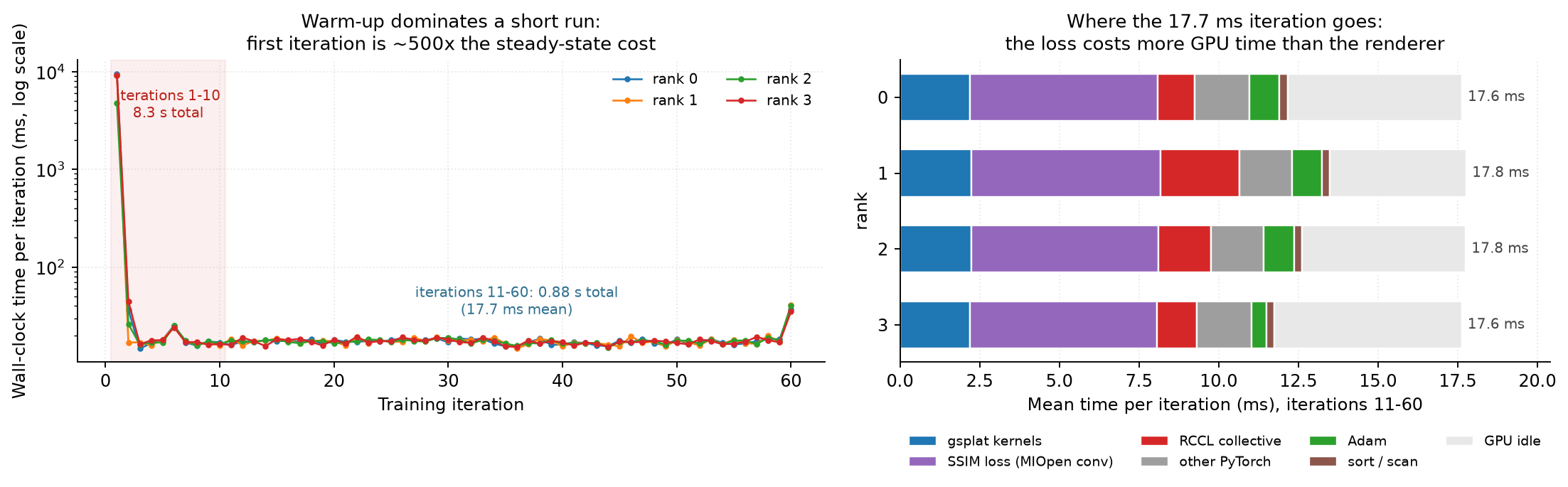
Figure 4: Left, wall-clock time per iteration on all four ranks (log scale). Right, the steady-state iteration budget per rank, broken down by kernel category, with time when the GPU had no work queued shown in grey.

Averaged over the four ranks and over iterations 11 to 60, the 17.70 ms iteration divides up like this:

Component	Time	Share of iteration
SSIM term of the loss (MIOpen convolutions)	5.88 ms	33%
gsplat kernels (project, evaluate SH, intersect, rasterize)	2.23 ms	13%
RCCL collectives	1.64 ms	9%
Other PyTorch elementwise, reduction, and copy kernels	1.68 ms	9%
Adam	0.83 ms	5%
Radix sort and scan over tile-Gaussian keys	0.25 ms	1%
GPU idle, nothing queued	5.19 ms	29%
Total	17.70 ms	100%

Aggregate throughput in the steady state is 226 images per second across the four GPUs. The median iteration takes 17.4 ms and nine out of ten finish within 18.7 ms.

Three things in that table are worth dwelling on, because none of them is what you would guess before profiling.

Communication is not the bottleneck at this scale. RCCL accounts for 9% of the iteration. In the default dense path the exchanged volume grows as \(48 \times N_r \times C_{\text{local}} \times (W - 1)\) bytes, and with only 13,569 Gaussians per rank there is very little to move. That fraction climbs steeply at production Gaussian counts, which is exactly when --packed starts to pay for itself — but on a small scene, tuning the interconnect is time wasted.

The loss costs more GPU time than the renderer. 5.88 ms against 2.23 ms, more than two to one. The convolutions come from the SSIM term: two MIOpen Winograd convolutions per iteration at roughly 2.9 ms each, wrapped in reflection padding. That is the signature of a convolution-based SSIM rather than of the fused one — the trace contains no fusedssim kernel at all, even though simple_trainer.py calls fused_ssim by default. MIOpen convolutions in the loss phase are therefore a reliable sign that the fused kernel is not being used, and getting it back hands most of those 5.9 ms to the renderer. This is the single largest optimization available in this trace, and it has nothing to do with distribution.

The GPU is idle for 29% of the step. With a single roughly one-million-pixel camera per rank, most kernels finish in tens of microseconds and the Python and launch overhead between them is not hidden. This is the concrete argument for raising --batch_size, which is discussed in the next section: more views per rank per step means larger kernels and proportionally less launch overhead, not just more images consumed.

Skew, and Where It Hides

The four ranks look perfectly balanced if you only look at step time. Their steady-state means are 17.63, 17.77, 17.75, and 17.63 ms — within 0.8% of each other. That balance is an artifact of synchronization, not evidence that the work was equal.

• Per iteration, the gap between the fastest and slowest rank averages 1.63 ms and reaches 5.65 ms, roughly a third of an iteration.

• Time spent inside RCCL device kernels varies by 2.1x across ranks, from 1.18 to 2.49 ms per iteration, while total step time varies by 0.8%. The collectives are absorbing the skew as wait time.

• The underlying cause is visible directly. intersect_offset_kernel is launched with one thread per tile-Gaussian intersection, so its grid size is a free measurement of how much rasterization work a camera implies. Across the 240 (rank, iteration) samples it ranges from 527 thousand to 2.26 million intersections, a 4.3x spread. Within a single step, the busiest rank averages 1.74x the intersections of the quietest, and in the worst step the ratio is 3.41x.

This is the “no pixel-level load balancing” limitation, measured. It matters for how you read a profile: when ranks show matching step times but very different communication times, the problem is camera-dependent work, not the transport. Tuning RCCL will not help.

One related observation. On every rank, the union of all kernel intervals equals the sum of their durations, so no two kernels ever ran concurrently and none of the 1.64 ms of RCCL time was hidden behind compute. That is structural rather than a configuration mistake: the payload exchange sits on the critical path between the Gaussian-parallel projection and the camera-parallel rasterization, and there is no independent work available to overlap with it. It is the exact inverse of DDP, where bucketing exists precisely so that gradient all-reduces can hide behind the remaining backward pass.

Warm-Up Costs More Than the Run

The left panel of Figure 4 is on a log scale for a reason. The first iteration takes 8.14 s on average and 9.50 s on the slowest rank, of which 3.42 s is spent inside RCCL device kernels while connections, channels, and buffers are established on first touch. The second iteration takes 31 ms, the third takes 16 ms, and from there the run is in steady state. Before any of that, ncclCommInitRankConfig occupies 2.6 s per rank, and at the end ncclCommDestroy costs another 220 ms.

The arithmetic is worth stating plainly: iterations 1 to 10 account for 8.31 s of wall clock, and iterations 11 to 60 account for 0.88 s. Ninety percent of the training time in this capture went into the first sixth of the steps. In a real 30,000-step job this is amortized into nothing, but it makes short benchmarks meaningless. If you are comparing world sizes, discard at least the first ten iterations, and treat any measurement of fewer than a few hundred steps as a measurement of RCCL bootstrap.

Batching and Hyperparameter Scaling

gsplat’s simple_trainer.py defaults to batch_size = 1, which means one camera view per rank per step. That is the historical 3DGS convention, and it is a poor fit for a distributed run: with only one view in flight per GPU, there is not much work to hide communication behind. Increasing batch_size gives each rank several views per step, which amortizes the fixed cost of the exchange over more useful rasterization work.

The effective global batch is the product of both factors, and gsplat computes it explicitly:

# examples/simple_trainer.py, create_splats_with_optimizers()
BS = batch_size * world_size
optimizers = {
    name: optimizer_class(
        [{"params": splats[name], "lr": lr * math.sqrt(BS), "name": name}],
        eps=1e-15 / math.sqrt(BS),
        betas=(1 - BS * (1 - 0.9), 1 - BS * (1 - 0.999)),
    )
    for name, _, lr in params
}

Three adjustments are applied automatically, so you do not need to retune anything when you add GPUs:

• Learning rates scale as \(\sqrt{\text{BS}}\). The familiar linear scaling rule is derived for SGD. Adam already divides by the square root of the second-moment estimate, which absorbs part of the batch-size effect, leaving a square-root rather than linear dependence.

• Adam’s \(\varepsilon\) scales as \(1/\sqrt{\text{BS}}\), keeping it in proportion to the rescaled updates.

• The momentum coefficients are decayed so that the effective averaging window shrinks as the batch grows. A larger batch already averages over more views, so the optimizer should lean less on history. Note that this linearization becomes degenerate at large BS: at BS = 10, \(\beta_1\) reaches zero. The source flags this as a known limitation, so treat very large effective batch sizes with care.

Because the learning-rate schedules and the densification intervals are all expressed in steps, adding GPUs without touching max_steps means the job consumes world_size times more images. The --steps_scaler flag exists to correct for this and is applied to every step-dependent hyperparameter at once:

# examples/simple_trainer.py, Config.adjust_steps()
def adjust_steps(self, factor: float):
    self.eval_steps = [int(i * factor) for i in self.eval_steps]
    self.save_steps = [int(i * factor) for i in self.save_steps]
    self.ply_steps = [int(i * factor) for i in self.ply_steps]
    self.max_steps = int(self.max_steps * factor)
    self.sh_degree_interval = int(self.sh_degree_interval * factor)

    strategy = self.strategy
    if isinstance(strategy, DefaultStrategy):
        strategy.refine_start_iter = int(strategy.refine_start_iter * factor)
        strategy.refine_stop_iter = int(strategy.refine_stop_iter * factor)
        strategy.reset_every = int(strategy.reset_every * factor)
        strategy.refine_every = int(strategy.refine_every * factor)

This is the single most important flag to understand when reading scaling results, as the next section shows.

What You Actually Gain

The clearest benefit is memory. Because rank \(r\) allocates parameters and Adam state only for its own shard, per-rank memory falls close to

\[ \text{Memory per GPU} \approx \frac{\text{Total memory}}{\text{world size}} \]

and the total number of Gaussians a job can hold rises roughly linearly with GPU count. Figure 5 shows this on MI300X: memory per rank drops from 12.5 GB on a single GPU to 4.2 GB across 8 GPUs, with Gaussians per rank falling correspondingly.

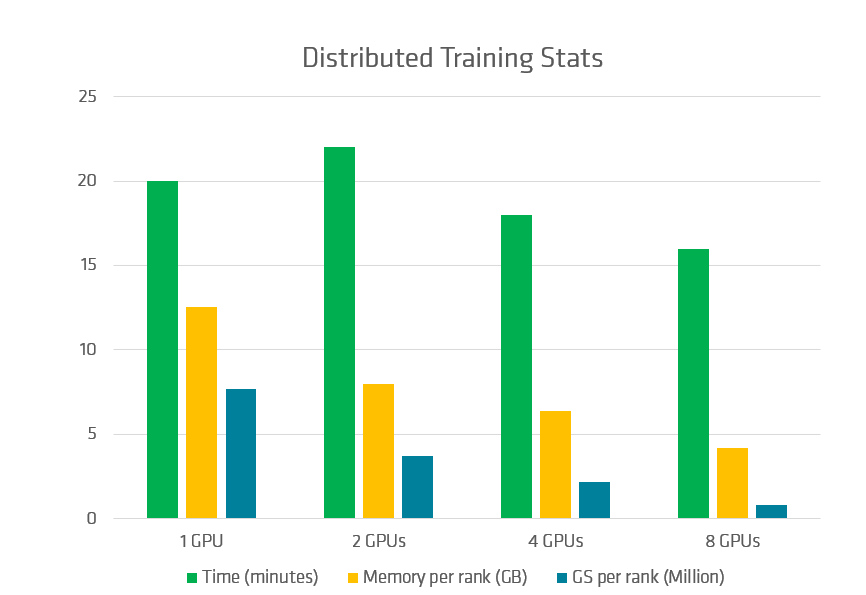
Figure 5: Distributed training statistics on MI300X. Memory and Gaussians per rank fall roughly as 1/world_size. Wall-clock time is nearly flat because these runs used a fixed step count.

The wall-clock bars in Figure 5 deserve a direct explanation, because at first glance they look like a scaling failure: 8 GPUs finish in 16 minutes against 20 minutes for one GPU, and 2 GPUs are actually slower than 1.

These runs used the default max_steps with no --steps_scaler. At a fixed step count, an \(n\)-GPU job consumes \(n\) times as many camera views as a single-GPU job, because every rank pulls its own view at every step. The 8-GPU run therefore processed eight times the training images in 0.8x the time, which is a throughput improvement of roughly 10x, not the 1.25x the bars suggest. The 2-GPU case looks worst because it pays the full price of admission — process group setup, per-step all_gather and all_to_all, index rebasing — while activating only a small fraction of the node’s xGMI links, and it recovers only a 2x increase in images consumed.

The practical reading is therefore:

• To increase capacity or throughput, add GPUs and keep max_steps fixed. You train on proportionally more views in roughly the same wall clock.

• To reduce wall-clock time to the same result, add GPUs and set --steps_scaler to the reciprocal of the GPU count. Four GPUs at --steps_scaler 0.25 see the same total number of images as the single-GPU baseline, in a fraction of the time.

• Prefer the full node. RCCL collectives are most efficient with all 8 GPUs participating, so an 8-GPU run has better communication efficiency than a 2- or 4-GPU run, not merely more of it.

• Profile before blaming the interconnect. The default dense exchange does send every local Gaussian to every peer regardless of visibility, and --packed fixes that. But in the 4-GPU trace above, communication was only 9% of the iteration while the loss was 33% and the GPU sat idle for another 29%. Confirm where the time actually goes before optimizing the part that sounds most expensive.

The quality benefit follows from the capacity benefit rather than from any change to the algorithm. On a single GPU you are forced to prune and densify conservatively to stay inside memory, and reconstruction quality on large high-resolution captures is still improving at the point where that limit bites. Distributing removes the constraint and lets adaptive density control run to its natural conclusion, so the gain shows up as higher PSNR and SSIM at convergence rather than as a faster step.

Running Distributed Training

The prerequisites and installation steps are covered in the previous gsplat post; in short, start from a ROCm PyTorch container and pip install amd_gsplat from the AMD-hosted index. Once the Mip-NeRF 360 dataset is downloaded, a single-GPU baseline looks like this:

CUDA_VISIBLE_DEVICES=0 python simple_trainer.py default \
    --data_dir data/360_v2/bicycle/ --data_factor 4 \
    --result_dir ./results/bicycle_1gpu

Scaling out requires no launcher and no code changes. gsplat.distributed.cli inspects CUDA_VISIBLE_DEVICES, spawns one worker per visible device with torch.multiprocessing.spawn, picks a free port for the rendezvous, and initializes the RCCL process group itself. You simply list more devices:

# Distributed training on 4 GPUs.
# The effective batch size is 4x larger, so scale the step count down to
# see the same total number of images as the single-GPU run.
CUDA_VISIBLE_DEVICES=0,1,2,3 python simple_trainer.py default \
    --data_dir data/360_v2/bicycle/ --data_factor 4 \
    --result_dir ./results/bicycle_4gpu \
    --steps_scaler 0.25

To spend the extra GPUs on reconstruction quality rather than on wall clock, use the whole node, leave --steps_scaler alone, and raise --batch_size so each rank has more views per step to hide communication behind:

CUDA_VISIBLE_DEVICES=0,1,2,3,4,5,6,7 python simple_trainer.py default \
    --data_dir data/360_v2/bicycle/ --data_factor 4 \
    --result_dir ./results/bicycle_8gpu \
    --batch_size 2 --packed

Because cli also recognizes the OpenMPI environment variables (OMPI_COMM_WORLD_SIZE, OMPI_COMM_WORLD_RANK, and OMPI_COMM_WORLD_LOCAL_RANK), the same script scales past one node under mpirun with no code changes:

mpirun -np 16 --hostfile hosts.txt --bind-to numa \
    python simple_trainer.py default \
    --data_dir data/360_v2/bicycle/ --data_factor 4 \
    --result_dir ./results/bicycle_multinode \
    --steps_scaler 0.0625

A few things about the output are specific to distributed runs:

• Checkpoints are per rank. Each rank writes ckpts/ckpt_<step>_rank<r>.pt containing only its own shard. After the final step, rank 0 concatenates them and exports a single merged point_cloud_<step>_distributed_merged.ply for viewing or downstream use.

• Statistics are per rank. stats/train_step<step>_rank<r>.json reports that rank’s peak memory and local Gaussian count, which is what Figure 5 plots. Multiply by world_size for scene totals.

• The interactive viewer is disabled. main() forces disable_viewer = True when world_size > 1 and prints a notice. Use the merged .ply in a standalone viewer instead.

• Evaluation renders on all ranks but reports from rank 0. Every rank participates in the distributed rasterization of the validation views, and rank 0 writes the images, metrics, and TensorBoard scalars.

Known Limitations

Distributed mode in gsplat is production-usable but not unconstrained. The current release enforces or omits the following:

• AbsGrad is unsupported. rasterization() asserts not distributed when absgrad=True, so the AbsGS densification variant is single-GPU only.

• Only per-Gaussian colors are allowed. Per-camera color tensors and the newer batched rendering API (batch_dims) are both rejected in distributed mode.

• Shards are never rebalanced. Densification is purely local, so ranks whose region of the scene happens to densify faster accumulate more Gaussians and more work. Nothing redistributes them, and the slowest rank sets the pace of every step.

• There is no pixel-level load balancing. Work is partitioned at camera granularity, so a rank that draws a detail-dense view does more work that step than a rank that draws sky. In the trace above this showed up as a 4.3x range in tile-Gaussian intersection counts and a 2.1x range in per-rank communication time. The imbalance averages out over many steps rather than being corrected within one.

• Communication is fully exposed. The Gaussian exchange sits on the critical path between the two parallel stages, so unlike a DDP gradient all-reduce it cannot be overlapped with computation. The trace shows no kernel concurrency at all.

• The interactive viewer is unavailable, as noted above.

The first two are explicit assertions you will hit immediately. The rest are performance characteristics rather than errors, and they are the main reason measured scaling falls short of ideal.

Potential Use Cases

• Large-scale digital twins of cities, industrial sites, and heritage locations, where the capture area alone puts the Gaussian count out of single-GPU reach.

• VR and AR streaming, where preserving fine detail matters and decimating the scene to fit is not acceptable.

• Film and VFX, where full-resolution splats can be trained without the quality compromise that pruning imposes.

• Autonomous driving, where street-level reconstructions are trained from large dashcam corpora and turnaround time directly limits iteration speed.

Summary

Gaussian splatting scales beautifully until it does not. A single Gaussian costs a few hundred bytes once Adam state is included, so a single MI300X saturates at a few hundred million primitives — and on large high-resolution captures, quality is still climbing when you get there. That makes single-GPU training both limiting and lossy.

gsplat’s answer is a mixed-parallelism scheme rather than conventional data parallelism. Gaussians are split across ranks with a strided round-robin partition and never replicated, so parameters and optimizer state shard cleanly and per-rank memory falls as \(1/\text{world size}\). Projection runs Gaussian-parallel over all cameras; an all_to_all routes the projected Gaussian records to whichever rank owns the camera that needs them; rasterization and loss run camera-parallel; and gradients return through the transpose of that same exchange. Nothing about the scene is ever all-reduced. PyTorch DDP appears only around the small auxiliary pose and appearance modules, and RCCL provides the transport over xGMI.

A trace of a 4-GPU run confirms all of that in numbers: five collectives per iteration, two metadata all-gathers and three grouped all-to-alls, and exactly one ncclAllReduce in a 34.7-second capture that lands after the last training step. It also punctures a few assumptions. Communication was 9% of the iteration, the SSIM term of the loss was 33%, and the GPU had nothing queued for another 29%. Ninety percent of the wall clock went into the first ten of sixty steps, spent bootstrapping RCCL.

Three things are worth carrying away when you read scaling numbers. First, gsplat’s distributed mode primarily buys capacity and throughput; wall-clock time only falls if you scale max_steps down with --steps_scaler. Second, communication efficiency is best when all eight GPUs on a node participate, so small multi-GPU configurations understate what the approach can do. Third, profile before you optimize: on a scene small enough to fit one GPU, the interconnect is rarely the thing standing in your way.

The future of gsplat is not just faster. It is distributed. In this blog, we explored why single-GPU 3DGS training hits a memory wall, how gsplat partitions the workload across GPUs, and how RCCL collectives coordinate the distributed pipeline on AMD Instinct™ GPUs. You also learned how to reason about memory growth, identify the bottlenecks that matter, and validate a real four-GPU run with rocprofv3.

Additional Resources

• gsplat for ROCm on GitHub and the gsplat documentation

• Understanding RCCL Bandwidth and xGMI Performance on AMD Instinct MI300X

• RCCL on GitHub and rccl-tests

• rocprofv3 and the rocprofiler SDK, used to capture the trace behind Figures 2 and 3, and the Perfetto UI for viewing it

• PyTorch Distributed Data Parallel notes

• Ye, Vickie, Ruilong Li, Justin Kerr, Matias Turkulainen, Brent Yi, Zhuoyang Pan, Otto Seiskari et al. “gsplat: An open-source library for Gaussian splatting.” Journal of Machine Learning Research 26, no. 34 (2025): 1-17.

• Kerbl, Bernhard, Georgios Kopanas, Thomas Leimkühler, and George Drettakis. “3D Gaussian splatting for real-time radiance field rendering.” ACM Transactions on Graphics 42, no. 4 (2023): 139-1.

• Zhao, Hexu, Haoyang Weng, Daohan Lu, Ang Li, Jinyang Li, Aurojit Panda, and Saining Xie. “On Scaling Up 3D Gaussian Splatting Training.” 2024. The multi-GPU strategy in gsplat/rendering.py cites this work.

Disclaimers

The information presented in this document is for informational purposes only and may contain technical inaccuracies, omissions, and typographical errors. The information contained herein is subject to change and may be rendered inaccurate for many reasons, including but not limited to product and roadmap changes, component and motherboard version changes, new model and/or product releases, product differences between differing manufacturers, software changes, BIOS flashes, firmware upgrades, or the like. Any computer system has risks of security vulnerabilities that cannot be completely prevented or mitigated. AMD assumes no obligation to update or otherwise correct or revise this information. However, AMD reserves the right to revise this information and to make changes from time to time to the content hereof without obligation of AMD to notify any person of such revisions or changes. THIS INFORMATION IS PROVIDED ‘AS IS.” AMD MAKES NO REPRESENTATIONS OR WARRANTIES WITH RESPECT TO THE CONTENTS HEREOF AND ASSUMES NO RESPONSIBILITY FOR ANY INACCURACIES, ERRORS, OR OMISSIONS THAT MAY APPEAR IN THIS INFORMATION. AMD SPECIFICALLY DISCLAIMS ANY IMPLIED WARRANTIES OF NON-INFRINGEMENT, MERCHANTABILITY, OR FITNESS FOR ANY PARTICULAR PURPOSE. IN NO EVENT WILL AMD BE LIABLE TO ANY PERSON FOR ANY RELIANCE, DIRECT, INDIRECT, SPECIAL, OR OTHER CONSEQUENTIAL DAMAGES ARISING FROM THE USE OF ANY INFORMATION CONTAINED HEREIN, EVEN IF AMD IS EXPRESSLY ADVISED OF THE POSSIBILITY OF SUCH DAMAGES. AMD, the AMD Arrow logo, and combinations thereof are trademarks of Advanced Micro Devices, Inc. Other product names used in this publication are for identification purposes only and may be trademarks of their respective companies. © 2026 Advanced Micro Devices, Inc. All rights reserved